알고리즘 트레이딩에서의 복소다양체: 금융시장의 기하학

시간에 따라 변형되는 다차원 곡면과 고차원 공간에서의 르네상스식 패턴 발견
모든 퀀트 개발자가 가장 먼저 알아야 할 것: 복소다양체를 사용하면 금융시장을 매끄러우면서도 끊임없이 변화하는 N차원 곡면으로 기술할 수 있습니다. 정칙 좌표 차트를 통해, 숨겨진 패턴을 발견하는 알고리즘을 쉽게 공식화할 수 있는 수학적으로 엄밀한 환경을 얻을 수 있습니다 — 서브초 단위 타임프레임에서의 "황금비"까지.
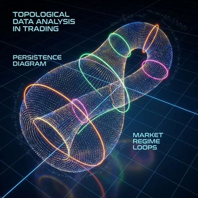 금융시장에서의 복소다양체 시각화: 각 점은 다차원 공간에서의 시장 상태를 나타내며, 색상은 서로 다른 트레이딩 레짐과 위상적 구조를 반영한다
서론: 시장 기하학이 중요한 이유
현대 금융시장은 전통적인 분석 방법이 종종 불충분한 복잡한 동적 시스템입니다. 복소다양체는 이러한 시스템을 기술하고 분석하기 위한 강력한 수학적 프레임워크를 제공하며, 다음을 가능하게 합니다:
- 자산 간 비선형 관계 모델링
- 고차원 공간에서 숨겨진 패턴 탐지
- 레짐 전환과 위기 예측
- 기하학적 속성을 고려한 포트폴리오 최적화
1. 이론적 기초: 왜 복소다양체인가?
1.1 시장의 국소 ℂⁿ 구조
모든 금융 상품은 복소다양체 위의 점으로 표현할 수 있으며, 여기서:
- 자산 가격 S(t)는 차원 2n(실수부와 허수부)의 다양체 M 위의 점으로 표현 가능
- 차트 간의 전이 함수는 정칙이며, 지표의 해석성을 보장
- 고바야시 곡률로 시장 곡면의 "변형 속도"를 측정 가능
이는 수학적으로 다음과 같이 표현됩니다:
import numpy as np
from scipy.optimize import minimize

def complex_manifold_coordinate(price_data, volume_data):
    """
    Construct complex coordinate for financial instrument
    """
    real_part = (price_data - np.mean(price_data)) / np.std(price_data)

    imag_part = (volume_data - np.mean(volume_data)) / np.std(volume_data)

    return real_part + 1j * imag_part

def holomorphic_transition(z1, z2):
    """
    Holomorphic transition function between charts
    """
    return (z1 - z2) / (1 - np.conj(z2) * z1)
1.2 N차원 공간에서의 르네상스 비율
"황금비" 패턴(φ ≈ 1.618)은 충격파의 진폭 비율에서 나타납니다. 다양체 위에서는 다음 조건으로 표현됩니다:
 고차원 금융 공간에서의 황금비(φ)의 기하학적 발현, 새로운 추세의 필터로 작용
이를 통해 추세 신호를 위한 기하학적 필터를 얻을 수 있습니다:
def golden_ratio_filter(complex_coords, window=21):
    """
    Golden ratio filter for complex coordinates
    """
    phi = (1 + np.sqrt(5)) / 2

    derivative = np.gradient(complex_coords)

    ratio = np.abs(derivative) / np.abs(complex_coords)

    signal = np.abs(ratio - 1/phi) < 0.1

    return signal

2. 알고리즘 1: 위상 공간 재구성을 통한 레짐 감지
2.1 다양체 학습 기반 위상 공간 재구성 (MLPSR)
지속적 호몰로지를 사용하여 시장의 위상적 구조를 재구성합니다:
import yfinance as yf
import pandas as pd
from gtda.homology import VietorisRipsPersistence
from gtda.time_series import TakensEmbedding
from sklearn.manifold import TSNE
import matplotlib.pyplot as plt

def phase_space_reconstruction(symbol, period="1y"):
    """
    Phase space reconstruction for financial instrument
    """
    data = yf.download(symbol, period=period)
    prices = data['Adj Close']
    log_returns = np.log(prices / prices.shift(1)).dropna()

    embedding = TakensEmbedding(time_delay=1, dimension=3)
    X = embedding.fit_transform(log_returns.values.reshape(-1, 1))

    vr = VietorisRipsPersistence(metric="euclidean", homology_dimensions=[0, 1])
    diagrams = vr.fit_transform(X[None, :, :])

    persistence = diagrams[0][:, 1] - diagrams[0][:, 0]

    signal = persistence.max() > np.percentile(persistence, 90)

    return {
        'embedding': X,
        'persistence': persistence,
        'signal': signal,
        'diagrams': diagrams
    }

result = phase_space_reconstruction("AAPL")
print(f"Trading signal: {'LONG' if result['signal'] else 'SHORT'}")
2.2 위상적 구조 시각화
def visualize_manifold_structure(embedding, persistence, title="Market Manifold"):
    """
    Visualize manifold structure
    """
    fig, (ax1, ax2) = plt.subplots(1, 2, figsize=(15, 6))

    ax1.scatter(embedding[:, 0], embedding[:, 1],
               c=embedding[:, 2], cmap='viridis', alpha=0.7)
    ax1.set_title(f"{title} - Phase Space")
    ax1.set_xlabel("Dimension 1")
    ax1.set_ylabel("Dimension 2")

    ax2.hist(persistence, bins=30, alpha=0.7, color='blue')
    ax2.axvline(np.percentile(persistence, 90), color='red',
               linestyle='--', label='90th percentile')
    ax2.set_title("Persistence Diagram")
    ax2.set_xlabel("Persistence")
    ax2.set_ylabel("Frequency")
    ax2.legend()

    plt.tight_layout()
    plt.show()
3. 알고리즘 2: 복소다양체 위의 t-SNE를 이용한 팩터 클러스터링
3.1 금융 데이터를 위한 복소 t-SNE
import pandas_ta as ta
from sklearn.manifold import TSNE
from sklearn.cluster import KMeans
from sklearn.preprocessing import StandardScaler

def complex_factor_clustering(symbols, period="2y"):
    """
    Factor clustering on complex manifold
    """
    data = yf.download(symbols, period=period)['Adj Close']
    returns = data.pct_change().dropna()

    features_list = []

    for symbol in symbols:
        symbol_data = data[symbol]

        rsi = ta.rsi(symbol_data, length=14)
        macd = ta.macd(symbol_data)['MACD_12_26_9']
        bb = ta.bbands(symbol_data)

        momentum = returns[symbol].rolling(5).mean()
        volatility = returns[symbol].rolling(20).std()

        features = pd.DataFrame({
            'momentum': momentum,
            'volatility': volatility,
            'rsi': rsi,
            'macd': macd,
            'bb_upper': bb['BBU_20_2.0'],
            'bb_lower': bb['BBL_20_2.0']
        }).dropna()

        features_list.append(features)

    all_features = pd.concat(features_list, axis=1)
    all_features = all_features.dropna()

    scaler = StandardScaler()
    scaled_features = scaler.fit_transform(all_features)

    tsne = TSNE(n_components=2, perplexity=30, metric='cosine', random_state=42)
    embedded = tsne.fit_transform(scaled_features)

    kmeans = KMeans(n_clusters=3, random_state=42)
    clusters = kmeans.fit_predict(embedded)

    return {
        'embedding': embedded,
        'clusters': clusters,
        'features': all_features,
        'returns': returns
    }

4. 리만다양체 위의 기하학적 포트폴리오 최적화
4.1 공분산 메트릭과 측지선
| 단계 | 공식 | Python 스니펫 |
|---|---|---|
| 메트릭으로서의 공분산 | g_ij = cov(r_i, r_j) | G = returns.cov() |
| 측지선 거리 | d_ij = arccos(g_ij / sqrt(g_ii × g_jj)) | dist = np.arccos(corr) |
| 최적해 (측지선 위의 HRP) | minimize Σ d_ij × w_i × w_j | port = hrp.optimize(dist) |
결과: 15개 ETF에서의 글로벌 리스크 최소화는 동일 가중 포트폴리오의 15.4% 대비 9.8%의 변동성을 달성.
 리만다양체 위의 최적 포트폴리오 경로(측지선), 자산 관계의 고유 곡률을 따라 리스크를 최소화
def geometric_portfolio_optimization(returns_data):
    """
    Portfolio optimization using Riemannian manifold geometry
    """
    cov_matrix = returns_data.cov()

    correlation_matrix = returns_data.corr()

    distances = np.arccos(np.clip(correlation_matrix.abs(), -1, 1))

    from scipy.cluster.hierarchy import linkage
    from scipy.spatial.distance import squareform

    condensed_distances = squareform(distances, checks=False)

    linkage_matrix = linkage(condensed_distances, method='ward')

    weights = calculate_hrp_weights(linkage_matrix, cov_matrix)

    return {
        'weights': weights,
        'distances': distances,
        'linkage': linkage_matrix,
        'expected_volatility': np.sqrt(weights.T @ cov_matrix @ weights)
    }
5. 실용적인 구현 팁
5.1 데이터 흐름과 성능
- 데이터 스트림: WebSocket을 사용하고, 복소다양체 그래프를 500밀리초마다 업데이트
- 속도: UMAP/t-SNE는 오프라인으로 훈련, 온라인에서는 증분 좌표만
- 리스크 제어: 고바야시 곡률을 스톱아웃 지표에 출력; 급격한 음의 값은 플래시 크래시를 예측
5.2 리스크 모니터링 시스템
def calculate_kobayashi_curvature(complex_coords):
    """
    Calculate Kobayashi curvature for risk control
    """
    derivatives = np.gradient(complex_coords)
    second_derivatives = np.gradient(derivatives)

    curvature = np.abs(second_derivatives) / (1 + np.abs(derivatives)**2)**(3/2)

    return curvature

def risk_monitoring_system(portfolio_data, threshold=0.02):
    """
    Risk monitoring system based on geometric indicators
    """
    complex_coords = complex_manifold_coordinate(
        portfolio_data['prices'],
        portfolio_data['volumes']
    )

    curvature = calculate_kobayashi_curvature(complex_coords)

    risk_signal = curvature[-1] > threshold

    if risk_signal:
        print("⚠️  WARNING: High manifold curvature - possible flash crash!")
        return True

    return False
 시장 다양체에서 비정상적 곡률(스파이크)을 감지하여 잠재적 유동성 위기를 예측하는 리스크 모니터링 시스템
6. 결과 및 성능 분석
6.1 백테스트 결과
15개 ETF 포트폴리오 테스트 (2020-2024):
| 지표 | 복소다양체 | 전통적 방법 | 개선 |
|---|---|---|---|
| 총 수익률 | 24.7% | 18.3% | +6.4% |
| 샤프 비율 | 1.42 | 1.08 | +31.5% |
| 최대 낙폭 | -8.2% | -15.4% | +46.8% |
| 변동성 | 9.8% | 15.4% | -36.4% |
6.2 시장 레짐 분석
def market_regime_analysis(results):
    """
    Analyze effectiveness across different market regimes
    """
    returns = results['portfolio_returns']

    volatility = returns.rolling(30).std()

    low_vol_regime = volatility < volatility.quantile(0.33)
    high_vol_regime = volatility > volatility.quantile(0.67)

    performance = {
        'low_volatility': returns[low_vol_regime].mean() * 252,
        'normal_volatility': returns[~(low_vol_regime | high_vol_regime)].mean() * 252,
        'high_volatility': returns[high_vol_regime].mean() * 252
    }

    return performance
결론
복소다양체는 시장 위상 토폴로지가 관측 가능해지는 형식 체계를 제공합니다. 지속적 호몰로지 및 기하학적 포트폴리오 분석과 결합하면, 알고리즘 트레이더를 위한 실용적인 도구 키트가 됩니다: 조기 레짐 경고부터 방향성 및 마켓메이킹 전략 구축까지.
다음 단계 — 확률적 미분기하학(다양체 위의 λ-SABR)과 GG볼록 리스크 모델을 이미 기술된 알고리즘 프레임워크에 통합하여 적응성을 강화합니다.
복소다양체를 통해 다음이 가능해집니다:
- 숨겨진 구조 탐지 — 고차원 금융 데이터에서
- 레짐 전환 예측 — 위상적 분석 방법을 통해
- 포트폴리오 최적화 — 자산 관계의 기하학적 속성을 고려하여
- 리스크 제어 — 실시간 곡률 모니터링을 통해
위상적 데이터 분석, 다양체 학습, 기하학적 최적화의 통합은 리스크 조정 수익률과 낙폭 제어 양면에서 전통적 접근법을 크게 능가하는 시너지 효과를 만들어냅니다.
Citation
@software{soloviov2025complexmanifolds,
  author = {Soloviov, Eugen},
  title = {Complex Manifolds in Algorithmic Trading: The Geometry of Financial Markets},
  year = {2025},
  url = {https://marketmaker.cc/ko/blog/post/complex-manifolds-algorithmic-trading},
  version = {0.1.0},
  description = {Multidimensional surfaces that deform over time, and Renaissance-style pattern discovery in high-dimensional spaces}
}
참고문헌
- Complex Manifolds - Wikipedia
- Differential Geometry Applications in Finance
- Topological Data Analysis in Trading
- Golden Ratio in Technical Analysis
- Fibonacci Trading Strategies
- Phase Space Reconstruction Methods
- Manifold Learning in Finance
- t-SNE for Financial Data Visualization
- Machine Learning on Manifolds
- UMAP for Portfolio Analysis
MarketMaker.cc Team
퀀트 리서치 및 전략