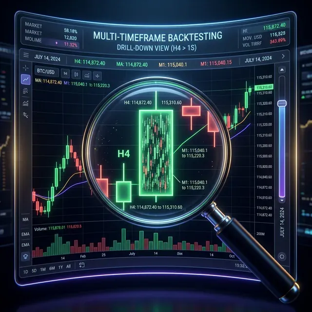
Adaptive Drill-Down: Backtest with Variable Granularity from Minutes to Raw Trades
Minute candles are the standard granularity for backtests. But within a single minute candle, price can move differently: sometimes by 0.01%, other times by 2%. When both stop-loss and take-profit fall within the [low, high] range of a single minute candle, the backtest doesn't know which triggered first. This is the fill ambiguity problem.
The naive solution is to switch to second-level data for the entire backtest. But over two years, that's ~63 million second bars instead of ~1 million minute bars. Storage increases 60x, speed drops proportionally.
Adaptive drill-down solves this problem: use fine granularity only where it's actually needed.
The Problem: Fill Ambiguity on Large Candles
Consider a specific situation. The strategy opened a long at 3000 USDT. Stop-loss: 2970 (-1%). Take-profit: 3060 (+2%).
The minute candle at 14:37:
- Open: 3010
- High: 3065
- Low: 2965
- Close: 3050
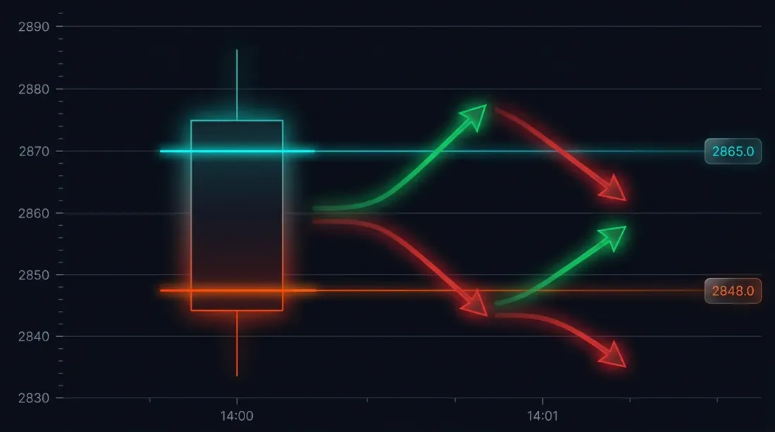
Both SL (2970) and TP (3060) fall within the range [2965, 3065]. Which triggered first?
Possible outcomes:
- Price went down first -> SL triggered -> loss of -1%
- Price went up first -> TP triggered -> profit of +2%
The difference in a single trade: 3 percentage points. With 10x leverage — 30%. For a backtest with hundreds of trades, incorrect fill ambiguity resolution systematically distorts results.
How Frameworks Handle This by Default
Most backtest engines use one of two heuristics:
- Optimistic: TP triggers first -> inflated results
- Pessimistic: SL triggers first -> deflated results
Both approaches are guesswork. Real data is available at second or even millisecond level, and there's no reason to guess when you can look.
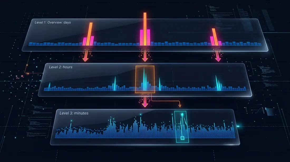
Drill-Down: Four-Level Strategy

The drill-down idea: start at the minute level and "drill down" to a lower level only when there's ambiguity — either due to price movement or volume spikes.
Level 1: 1m (minute candles)
  -> If SL or TP is unambiguously outside the [low, high] range — resolve on the spot
  -> If both are within the range — drill down

Level 2: 1s (second candles)
  -> Load 60 second bars for this minute
  -> Walk through second by second: which triggered first?
  -> If a second bar is ambiguous, OR price_move >= min_pct, OR volume >= median_1s * vol_mult — drill down

Level 3: 100ms (millisecond candles)
  -> Load up to 10 bars of 100ms for this second
  -> Walk through 100ms by 100ms
  -> If a 100ms bar is ambiguous, OR price_move >= min_pct, OR volume >= median_100ms * vol_mult — drill down

Level 4: Raw trades
  -> Load individual trades for this 100ms bucket
  -> Resolve the fill at trade-by-trade level — maximum possible precision
When Drill-Down Is Not Needed
In 95% of cases, drill-down is not required. Typical scenarios:
Unambiguous SL: candle high doesn't reach TP, low breaks through SL -> SL triggered, no drill-down needed.
Unambiguous TP: low doesn't reach SL, high breaks through TP -> TP triggered, no drill-down needed.
Neither triggered: both levels are outside the range -> position remains open.
Gap detection: the open of the next candle jumps through SL or TP -> execution at open price, no drill-down.
Drill-down is needed only for ~5% of bars — when both levels fall within the range of a single candle.
class AdaptiveFillSimulator:
    """
    Four-level drill-down for determining fill order.
    """
    def __init__(self, data_loader):
        self.loader = data_loader
        self.cache_1s = {}  # Cache of second data by month

    def check_fill(self, timestamp, candle_1m, sl_price, tp_price, side):
        """
        Checks whether SL or TP triggered on the given minute candle.

        Returns: ('sl', fill_price) | ('tp', fill_price) | None
        """
        low, high = candle_1m['low'], candle_1m['high']

        open_price = candle_1m['open']
        if side == 'long':
            if open_price <= sl_price:
                return ('sl', open_price)
            if open_price >= tp_price:
                return ('tp', open_price)
        else:
            if open_price >= sl_price:
                return ('sl', open_price)
            if open_price <= tp_price:
                return ('tp', open_price)

        sl_hit = self._level_hit(sl_price, low, high, side, 'sl')
        tp_hit = self._level_hit(tp_price, low, high, side, 'tp')

        if sl_hit and not tp_hit:
            return ('sl', sl_price)
        if tp_hit and not sl_hit:
            return ('tp', tp_price)
        if not sl_hit and not tp_hit:
            return None

        return self._drill_down_1s(timestamp, sl_price, tp_price, side)

    def _drill_down_1s(self, minute_ts, sl_price, tp_price, side):
        """Level 2: second-by-second pass."""
        bars_1s = self.loader.load_1s_for_minute(minute_ts)

        if bars_1s is None or len(bars_1s) == 0:
            return self._pessimistic_fill(side, sl_price, tp_price)

        for bar in bars_1s:
            sl_hit = self._level_hit(sl_price, bar['low'], bar['high'], side, 'sl')
            tp_hit = self._level_hit(tp_price, bar['low'], bar['high'], side, 'tp')

            if sl_hit and not tp_hit:
                return ('sl', sl_price)
            if tp_hit and not sl_hit:
                return ('tp', tp_price)
            if sl_hit and tp_hit:
                result = self._drill_down_100ms(bar['timestamp'], sl_price, tp_price, side)
                if result:
                    return result

        return self._pessimistic_fill(side, sl_price, tp_price)

    def _pessimistic_fill(self, side, sl_price, tp_price):
        """Pessimistic assumption: SL for longs, TP for shorts."""
        if side == 'long':
            return ('sl', sl_price)
        else:
            return ('sl', sl_price)
Performance
| Mode | Time per fill check | When used |
|---|---|---|
| 1m (no drill-down) | ~0ms | ~95% of cases |
| 1s drill-down | ~5ms (first access to month) | ~5% of cases |
| 100ms drill-down | ~1ms | <0.5% of cases |
| Raw trades drill-down | ~0.5ms | <0.1% of cases |
Over a 2-year backtest with ~400 trades, drill-down is invoked for approximately 20 candles. Total overhead — less than 1 second for the entire backtest.
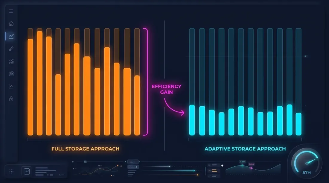
Adaptive Data Storage
Drill-down requires second and millisecond data. But storing everything at maximum granularity is impractical:
| Granularity | Bars over 2 years | Parquet size |
|---|---|---|
| 1m | ~1.05M | ~15 MB |
| 1s | ~63M | ~550 MB/month |
| 100ms | ~630M | ~5 GB/month |
A complete 1s archive over 2 years is about 13 GB. 100ms — over 100 GB. Storing everything is possible but wasteful, considering that drill-down uses less than 1% of this data.
Hot-Second Detection
The key observation: seconds in which price moves significantly represent a small fraction. If price changed by less than 0.1% within a second — there's no point storing the 100ms breakdown for that second.
Hot-second detection: when downloading and processing data, we analyze each second and generate 100ms candles only for "hot" seconds — those where price movement exceeded the threshold.
def process_trades_adaptive(
    trades: pd.DataFrame,
    min_price_change_pct: float = 1.0,
) -> tuple[pd.DataFrame, pd.DataFrame]:
    """
    Processes raw trades into an adaptive structure:
    - 1s candles for all seconds
    - 100ms candles only for "hot" seconds

    Args:
        trades: DataFrame with columns [timestamp, price, quantity]
        min_price_change_pct: threshold for drill-down to 100ms

    Returns:
        (df_1s, df_100ms_hot) — second candles and 100ms for hot seconds
    """
    trades['second'] = trades['timestamp'].dt.floor('1s')
    df_1s = trades.groupby('second').agg(
        open=('price', 'first'),
        high=('price', 'max'),
        low=('price', 'min'),
        close=('price', 'last'),
        volume=('quantity', 'sum'),
    )

    df_1s['price_change_pct'] = (df_1s['high'] - df_1s['low']) / df_1s['open'] * 100
    hot_seconds = df_1s[df_1s['price_change_pct'] >= min_price_change_pct].index

    hot_trades = trades[trades['second'].isin(hot_seconds)]
    hot_trades['bucket_100ms'] = hot_trades['timestamp'].dt.floor('100ms')

    df_100ms = hot_trades.groupby('bucket_100ms').agg(
        open=('price', 'first'),
        high=('price', 'max'),
        low=('price', 'min'),
        close=('price', 'last'),
        volume=('quantity', 'sum'),
    )

    return df_1s, df_100ms
Storage Savings
For example — ETHUSDT over a typical month:
| Approach | Size | Granularity |
|---|---|---|
| 1m only | ~1 MB | 1 minute |
| All 1s | ~550 MB | 1 second |
| All 100ms | ~5 GB | 100 ms |
| Adaptive | ~600 MB | 1s + 100ms only for hot seconds |
With a threshold of min_price_change_pct = 1.0%, hot seconds account for less than 1% of all seconds. 100ms data for them adds ~50 MB to the 550 MB of second data — a negligible overhead.
If second data is also stored adaptively (only when movement within a minute exceeds 0.1%), the volume can be reduced by another 3-5x.

Parquet Storage Structure
data/{SYMBOL}/
├── source.json                # Exchange source: {"exchange": "binance"} or {"exchange": "bybit"}
├── stats.json                 # Precomputed median volumes: {"median_volume_1s": ..., "median_volume_100ms": ...}
├── klines_1m/
│   ├── 2024-01.parquet       # ~1 MB
│   ├── 2024-02.parquet
│   └── ...
├── klines_1s/
│   ├── 2024-01.parquet       # ~550 MB
│   └── ...
├── klines_100ms_hot/
│   ├── 2024-01.parquet       # ~50 MB (hot seconds only)
│   └── ...
├── trades_hot/
│   ├── 2024-01.parquet       # Raw trades for hot 100ms buckets
│   └── ...
└── states_1m.parquet          # Precomputed rolling state cache (~112 MB)
Each file covers one month of data. Second, millisecond, and trade data is loaded lazily — only when drill-down requests it. The stats.json file contains precomputed median volumes used for volume-based drill-down triggers.
Parquet Optimization for Financial Data
Financial data has specific characteristics: timestamps grow monotonically, prices change smoothly, volumes vary significantly. Optimal settings:
import pyarrow as pa
import pyarrow.parquet as pq

schema = pa.schema([
    pa.field("timestamp", pa.int32()),    # Seconds from epoch — int32 is sufficient
    pa.field("open",      pa.float32()),
    pa.field("high",      pa.float32()),
    pa.field("low",       pa.float32()),
    pa.field("close",     pa.float32()),
    pa.field("volume",    pa.float32()),
])

column_encodings = {
    "timestamp": "DELTA_BINARY_PACKED",   # Monotonic int -> delta compression
    "open":      "BYTE_STREAM_SPLIT",     # Float -> byte-stream split
    "high":      "BYTE_STREAM_SPLIT",
    "low":       "BYTE_STREAM_SPLIT",
    "close":     "BYTE_STREAM_SPLIT",
    "volume":    "BYTE_STREAM_SPLIT",
}

def save_optimized_parquet(df, path):
    table = pa.Table.from_pandas(df, schema=schema)
    pq.write_table(
        table, path,
        compression="zstd",
        compression_level=9,
        use_dictionary=False,
        write_statistics=False,
        column_encoding=column_encodings,
    )
Why these settings:
- DELTA_BINARY_PACKED for timestamps: consecutive timestamps differ by a fixed value (60 for 1m, 1 for 1s). Delta encoding compresses them to nearly zero.
- BYTE_STREAM_SPLIT for float: splits float32 bytes into streams (all first bytes together, all second bytes together, etc.). For smoothly changing prices, this achieves 2-3x better compression than standard encoding.
- ZSTD level 9: good compression with acceptable decompression speed.
- float32 instead of float64: sufficient for prices and volumes, saves 50% memory.
Lazy Loading with Caching
Drill-down requests second data for a specific minute. Loading a parquet file for each request is slow. The solution — lazy loading with an LRU cache by month.
from functools import lru_cache
import pyarrow.parquet as pq
import pandas as pd

class AdaptiveDataLoader:
    """
    Lazy loader with cache: loads second data by month,
    keeps the last N months in memory.
    """
    def __init__(self, symbol: str, data_dir: str = "data", cache_months: int = 2):
        self.symbol = symbol
        self.data_dir = data_dir
        self.cache_months = cache_months
        self._cache_1s: dict[str, pd.DataFrame] = {}

    def load_1s_for_minute(self, minute_ts: pd.Timestamp) -> pd.DataFrame | None:
        """Load 1s data for a specific minute."""
        month_key = minute_ts.strftime("%Y-%m")

        if month_key not in self._cache_1s:
            self._load_month_1s(month_key)

        if month_key not in self._cache_1s:
            return None

        df = self._cache_1s[month_key]
        minute_start = minute_ts.floor('1min')
        minute_end = minute_start + pd.Timedelta(minutes=1)

        return df[(df.index >= minute_start) & (df.index < minute_end)]

    def load_100ms_for_second(self, second_ts: pd.Timestamp) -> pd.DataFrame | None:
        """Load 100ms data for a hot second."""
        month_key = second_ts.strftime("%Y-%m")
        path = f"{self.data_dir}/{self.symbol}/klines_100ms_hot/{month_key}.parquet"

        try:
            df = pd.read_parquet(path)
            second_start = second_ts.floor('1s')
            second_end = second_start + pd.Timedelta(seconds=1)
            return df[(df.index >= second_start) & (df.index < second_end)]
        except FileNotFoundError:
            return None

    def _load_month_1s(self, month_key: str):
        """Load a month of 1s data, evict old data from cache."""
        path = f"{self.data_dir}/{self.symbol}/klines_1s/{month_key}.parquet"
        try:
            df = pd.read_parquet(path)
            df.index = pd.to_datetime(df['timestamp'], unit='s')

            if len(self._cache_1s) >= self.cache_months:
                oldest = min(self._cache_1s.keys())
                del self._cache_1s[oldest]

            self._cache_1s[month_key] = df
        except FileNotFoundError:
            pass
Applying Drill-Down to Backtesting
Integration into the backtest loop:
def backtest_with_adaptive_fill(
    states: pd.DataFrame,
    strategy_params: dict,
    data_loader: AdaptiveDataLoader,
) -> list:
    """
    Backtest with adaptive drill-down for fill simulation.
    """
    fill_sim = AdaptiveFillSimulator(data_loader)
    trades = []
    position = None

    for i in range(len(states)):
        row = states.iloc[i]
        ts = states.index[i]

        candle_1m = {
            'open': row['open'], 'high': row['high'],
            'low': row['low'], 'close': row['close'],
            'timestamp': ts,
        }

        if position is not None:
            fill = fill_sim.check_fill(
                ts, candle_1m,
                position['sl'], position['tp'],
                position['side'],
            )

            if fill is not None:
                fill_type, fill_price = fill
                trades.append({
                    'entry_time': position['entry_time'],
                    'exit_time': ts,
                    'side': position['side'],
                    'entry_price': position['entry_price'],
                    'exit_price': fill_price,
                    'exit_type': fill_type,
                    'drill_down': fill_sim.last_drill_depth,  # 0, 1, or 2
                })
                position = None
                continue

        signal = check_entry_signal(row, strategy_params)
        if signal and position is None:
            position = {
                'side': signal['side'],
                'entry_price': row['close'],
                'entry_time': ts,
                'sl': signal['sl'],
                'tp': signal['tp'],
            }

    return trades
Relationship with Rolling State Cache
Drill-down complements the aggregated parquet cache — they solve different problems:
| Rolling state cache | Adaptive drill-down | |
|---|---|---|
| Purpose | Correct HTF indicator values | Precise SL/TP execution order |
| Operates on | Every 1m candle | Only during fill ambiguity (~5%) |
| Data | Precomputed, stored permanently | Lazy loaded, cache of recent months |
| Affects | Entry/exit signals | Execution price and time |
Both approaches eliminate errors invisible at the daily candle level but critical for realistic backtesting.
Summary: Fill Simulation Approach Comparison
| Approach | Accuracy | Speed | Storage |
|---|---|---|---|
| OHLC heuristic (optimist/pessimist) | Low | Instant | 1m only |
| Full 1s backtest | High | Slow (x60) | ~550 MB/month |
| Full 100ms backtest | Very high | Very slow (x600) | ~5 GB/month |
| Full raw trades backtest | Maximum | Extremely slow | ~50 GB/month |
| Adaptive drill-down (4-level) | Maximum | ~Instant | 1m + 1s + 100ms hot + trades hot |
Drill-down provides the accuracy of a full 1s backtest at the speed of a 1m backtest. The key observation: high granularity is not needed everywhere — only at decision points.
Volume-Based Drill-Down
The original drill-down triggers only on price movement — when the [low, high] range of a candle is wide enough to create fill ambiguity. But price is not the only signal that something interesting happened within a bar.
Volume spikes are an equally important trigger. A second where volume is 500x the median typically corresponds to a large market order, a liquidation cascade, or a flash crash. Even if the candle body appears small, the actual price path within that second may have been wild — touching extremes that the OHLC representation hides.
The drill-down condition is now OR-based: either a significant price move OR an anomalous volume spike triggers the descent to finer granularity.
def is_hot(bar, median_volume, min_pct=0.1, vol_mult=500):
    """
    Determines if a bar warrants drill-down to the next level.
    Two independent triggers (OR logic):
      - price moved >= min_pct within the bar
      - volume exceeded median * vol_mult
    """
    price_move = (bar['high'] - bar['low']) / bar['open'] * 100
    return price_move >= min_pct or bar['volume'] >= median_volume * vol_mult
This catches scenarios invisible to price-only detection: a bar with open=3000, close=3001 but volume 50,000x the norm may have briefly touched 2950 and 3050 within milliseconds. Without volume-based drill-down, the backtest would never examine this second more closely.
Raw Trades: The Fourth Level
The original three-level hierarchy (1m -> 1s -> 100ms) still leaves a gap: within a single 100ms bucket, multiple trades can execute at different prices. For a bucket with high=3060 and low=2965, we still don't know the exact sequence.
The solution: drill down to raw trades as the fourth and final level.
1m candles (base)
  └─> 1s candles    (when 1s shows price_move >= min_pct OR volume >= median_1s * vol_mult)
      └─> 100ms candles  (when hot second detected)
          └─> Raw trades     (when 100ms shows price_move >= min_pct OR volume >= median_100ms * vol_mult)
At the raw trades level, there is no ambiguity — each trade has an exact price and timestamp. The fill is resolved definitively:
def resolve_from_trades(trades, sl_price, tp_price, side):
    """
    Walk through individual trades in chronological order.
    The first trade that crosses SL or TP determines the fill.
    """
    for trade in trades:
        price = trade['price']
        if side == 'long':
            if price <= sl_price:
                return ('sl', price)
            if price >= tp_price:
                return ('tp', price)
        else:  # short
            if price >= sl_price:
                return ('sl', price)
            if price <= tp_price:
                return ('tp', price)
    return None
The raw trades level is invoked extremely rarely — less than 0.1% of all bars — but when it is, it provides ground truth that no candle-based approximation can match.
Separate Thresholds per Transition
Different resolution transitions have different characteristics. A price move of 0.1% within a second is significant; the same 0.1% within a 100ms bucket is extreme. Similarly, volume distributions differ at each timescale.
Each level transition now has its own min_pct and vol_mult parameters:
1s → 100ms:   --min-pct-1s 0.1   --vol-mult-1s 500
100ms → trades: --min-pct-100ms 0.1 --vol-mult-100ms 500
This allows fine-tuning the sensitivity of each transition independently. In practice, the 100ms-to-trades transition can use a tighter threshold because the cost of loading raw trades for a single 100ms bucket is minimal.
@dataclass
class DrillDownConfig:
    min_pct_1s: float = 0.1
    vol_mult_1s: float = 500
    min_pct_100ms: float = 0.1
    vol_mult_100ms: float = 500
Persistent Median Statistics
Volume-based drill-down requires knowing the median volume at each timescale. Computing medians on-the-fly for every backtest would negate the performance benefits. The solution: precompute medians once and cache them.
For each symbol, median volumes at 1s and 100ms granularity are computed from historical data and stored in a stats.json file:
{
  "ETHUSDT": {
    "median_volume_1s": 12.5,
    "median_volume_100ms": 1.8
  },
  "BTCUSDT": {
    "median_volume_1s": 0.45,
    "median_volume_100ms": 0.06
  }
}
The statistics are computed once per symbol when data is first downloaded and reused across all subsequent backtests. If the data is updated (new months downloaded), the stats are recomputed incrementally.
def compute_median_stats(symbol, data_dir):
    """Compute and cache median volume stats for a symbol."""
    stats_path = f"{data_dir}/{symbol}/stats.json"

    all_1s = load_all_months(f"{data_dir}/{symbol}/klines_1s/")
    median_1s = all_1s['volume'].median()

    all_100ms = load_all_months(f"{data_dir}/{symbol}/klines_100ms_hot/")
    median_100ms = all_100ms['volume'].median()

    stats = {
        "median_volume_1s": float(median_1s),
        "median_volume_100ms": float(median_100ms),
    }

    with open(stats_path, 'w') as f:
        json.dump(stats, f, indent=2)

    return stats

Multi-Exchange Support: Bybit
Not all symbols are available on Binance. For assets like XAUTUSDT (gold), data must come from other exchanges. The drill-down system now supports Bybit as an alternative data source.
For Bybit symbols, all candle levels (1m, 1s, 100ms) and raw trades are built from Bybit's raw trade stream. The process is the same — raw trades are aggregated into candles at each timescale — but the data source differs.
data/{SYMBOL}/
├── source.json              # {"exchange": "bybit"} or {"exchange": "binance"}
├── klines_1m/
│   └── ...
├── klines_1s/
│   └── ...
├── klines_100ms_hot/
│   └── ...
└── trades_hot/              # Raw trades for hot 100ms buckets
    └── ...
The data loader checks source.json and uses the appropriate download pipeline. From the backtest engine's perspective, the data format is identical regardless of the source exchange — the drill-down logic is exchange-agnostic.
This is particularly important for cross-exchange strategies or symbols that trade exclusively on certain venues.
Conclusion
Adaptive drill-down is the application of a simple principle: spend computational resources and storage proportionally to data importance.
Four granularity levels:
- 1m — base pass for 95% of bars
- 1s — drill-down during fill ambiguity or volume spikes
- 100ms — drill-down for hot seconds with extreme movement or anomalous volume
- Raw trades — drill-down for hot 100ms buckets, resolving fills at individual trade level
Four storage levels:
- All 1m — complete archive, ~15 MB for 2 years
- All 1s — complete or adaptive archive, ~550 MB/month
- Hot 100ms only — <1% of seconds, ~50 MB/month
- Hot trades only — raw trades for the most extreme 100ms buckets
Two drill-down triggers (OR logic):
- Price-based: the bar's price range exceeds
min_pct - Volume-based: the bar's volume exceeds
median * vol_mult
The result: a backtest with tick simulator accuracy at minute-level speed. Storage that grows linearly, not exponentially. And support for multiple exchanges — Binance and Bybit — with exchange-agnostic drill-down logic.
For more on precomputed cache for multi-timeframe strategies, see the article Aggregated Parquet Cache. On the impact of funding rates on results with high leverage — Funding rates kill your leverage.
Useful Links
- Apache Parquet — data storage format
- Apache Arrow — BYTE_STREAM_SPLIT encoding
- Zstandard — compression algorithm
- Lopez de Prado — Advances in Financial Machine Learning
- Binance — Historical Market Data
Citation
@article{soloviov2026adaptivedrilldown,
  author = {Soloviov, Eugen},
  title = {Adaptive Drill-Down: Backtest with Variable Granularity from Minutes to Raw Trades},
  year = {2026},
  url = {https://marketmaker.cc/ru/blog/post/adaptive-resolution-drill-down-backtest},
  description = {How adaptive data granularity speeds up backtests and saves storage: drill-down from 1m to 1s, 100ms, and raw trades only where price moved significantly or volume spiked.}
}
MarketMaker.cc Team
Miqdoriy tadqiqotlar va strategiya
Read More

Aggregated Parquet Cache: How to Speed Up Multi-Timeframe Backtests by Hundreds of Times

Walk-Forward Optimization: The Only Honest Strategy Test