QuestDB for Algorithmic Trading: From Order Books to Production Architecture

Part 3 of 3 — also available in RU · ZH

Disclaimer: The information provided in this article is for educational and informational purposes only and does not constitute financial, investment, or trading advice. Trading cryptocurrencies involves significant risk of loss.

Welcome to the final part of our QuestDB series. In Part 1, we covered the storage architecture. In Part 2, we explored the SQL extensions. Now let's bring it all together: materialized views for real-time analytics, native order book storage with 2D arrays, and a reference architecture for a production algorithmic trading platform.

Materialized Views: Pre-Computed Analytics at Wire Speed

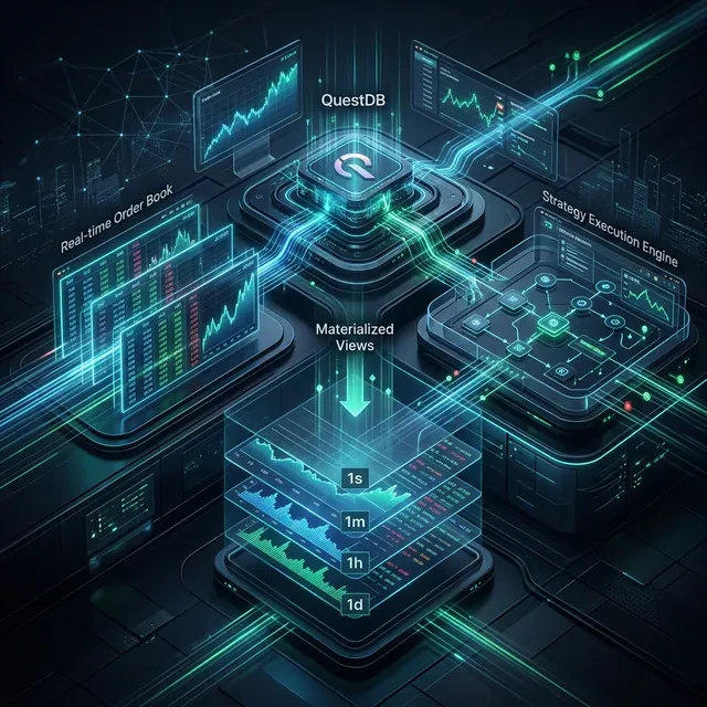
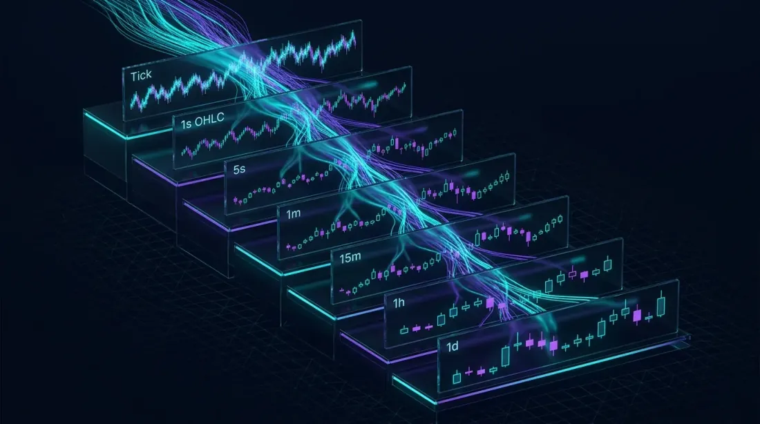Cascading materialized views: raw tick data flows through progressively coarser aggregation layers, each level processing a dramatically smaller dataset

If SAMPLE BY is QuestDB's most-used query, then materialized views are its most impactful optimization. The concept is simple: instead of computing OHLCV aggregations on every dashboard refresh or API call, pre-compute them once and keep the result continuously updated.

Basic OHLC Materialized View

CREATE MATERIALIZED VIEW trades_OHLC_15m
  WITH BASE 'trades'
  REFRESH IMMEDIATE
AS
SELECT timestamp, symbol,
  first(price) AS open,
  max(price) AS high,
  min(price) AS low,
  last(price) AS close,
  sum(quantity) AS volume
FROM trades
SAMPLE BY 15m;

That's the entire definition. Every time new rows are inserted into the trades table, QuestDB automatically and incrementally refreshes this view. Not a full recomputation — only the affected time buckets are updated. Queries against trades_OHLC_15m become simple lookups on a much smaller, pre-aggregated dataset.

The performance difference is dramatic. On a table with billions of rows, querying the base table for OHLC data might take 200ms. The materialized view returns the same result in under 5ms. With multiple concurrent dashboard users, this isn't just an optimization — it's the difference between a responsive system and one that falls over.

Cascaded Views: Multi-Timeframe from a Single Source

Here's where materialized views become architecturally elegant. You can chain them — each view feeds the next, creating a hierarchy of aggregation levels from a single raw data source:

-- 1-second bars from raw trades
CREATE MATERIALIZED VIEW ohlc_1s AS
SELECT timestamp, symbol,
  first(price) AS open, max(price) AS high,
  min(price) AS low, last(price) AS close,
  sum(quantity) AS volume
FROM trades
SAMPLE BY 1s;

-- 5-second bars from 1-second bars
CREATE MATERIALIZED VIEW ohlc_5s AS
SELECT timestamp, symbol,
  first(open) AS open, max(high) AS high,
  min(low) AS low, last(close) AS close,
  sum(volume) AS volume
FROM ohlc_1s
SAMPLE BY 5s;

-- 1-minute bars from 5-second bars
CREATE MATERIALIZED VIEW ohlc_1m AS
SELECT timestamp, symbol,
  first(open) AS open, max(high) AS high,
  min(low) AS low, last(close) AS close,
  sum(volume) AS volume
FROM ohlc_5s
SAMPLE BY 1m;

Each level processes a dramatically smaller dataset than the one before it. The 1-minute view doesn't scan raw trades — it only reads pre-aggregated 5-second bars. This cascading pattern scales to any number of timeframes: 1s → 5s → 1m → 5m → 15m → 1h → 4h → 1d.

For a crypto data platform ingesting from 100+ exchanges, this is the backbone of the entire OHLC delivery pipeline.

Refresh Strategies

QuestDB offers three refresh modes, each suited to different workloads:

REFRESH IMMEDIATE triggers an async refresh after every base table transaction. Best for real-time dashboards where sub-second latency matters.

REFRESH EVERY 1h (timer-based) batches updates into periodic refreshes. Better for high-throughput ingestion where triggering refresh on every micro-batch would create overhead.

REFRESH PERIOD (LENGTH 1d TIME ZONE 'Europe/London' DELAY 2h) defines calendar-aligned periods. The "delay" accounts for late-arriving data — critical for markets that might send correction feeds hours after the trading session.

REFRESH MANUAL gives full control. The view only updates when you explicitly run a REFRESH command — useful for end-of-day reconciliation workflows.

The LATEST ON Acceleration Pattern

One of the most powerful patterns combines materialized views with LATEST ON for instant portfolio snapshots. Scanning 1.3 billion raw rows for the latest price of each symbol takes seconds. But with a daily pre-aggregated view:

CREATE MATERIALIZED VIEW trades_latest_1d AS
SELECT timestamp, symbol, side,
  last(price) AS price,
  last(quantity) AS quantity,
  last(timestamp) AS latest
FROM trades
SAMPLE BY 1d;

The LATEST ON query scans roughly 25,000 pre-aggregated rows instead of billions:

SELECT symbol, side, price, quantity, latest AS timestamp
FROM (
  trades_latest_1d
  LATEST ON timestamp PARTITION BY symbol, side
)
ORDER BY timestamp DESC;

Seconds down to milliseconds. This is how production trading dashboards achieve real-time responsiveness over massive datasets.

TTL: Automatic Data Lifecycle

Materialized views support TTL (time-to-live) policies for automatic data expiration:

CREATE MATERIALIZED VIEW ohlc_1h AS (
  SELECT timestamp, symbol,
    avg(price) AS avg_price
  FROM trades
  SAMPLE BY 1h
) PARTITION BY WEEK TTL 8 WEEKS;

This keeps 8 weeks of hourly data, automatically dropping older partitions. Combined with the three-tier storage engine, you get a natural data lifecycle: raw ticks flow through WAL → columnar storage → Parquet on object storage, while materialized views maintain the pre-aggregated summaries your applications actually query.

2D Arrays: Native Order Book Analytics

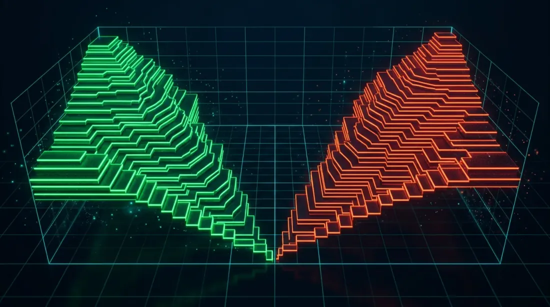3D order book depth: bid and ask levels stored as native 2D arrays, enabling SIMD-optimized spread calculations and liquidity analysis

QuestDB 9.0 introduced N-dimensional arrays — true shaped-and-strided, NumPy-like arrays that handle common operations (slicing, transposing) with zero copying. For trading, the killer application is order book storage.

The Traditional Problem

Historically, storing order book snapshots in a relational database was painful. You had two choices: one row per price level (explosion of rows, expensive to query depth), or a fixed number of columns like bid1_price, bid1_size, bid2_price, bid2_size, etc. (rigid, wasteful, and ugly).

QuestDB's 2D arrays eliminate both problems:

CREATE TABLE market_data (
  timestamp TIMESTAMP,
  symbol SYMBOL,
  bids DOUBLE[][],
  asks DOUBLE[][]
) TIMESTAMP(timestamp) PARTITION BY HOUR;

Each bids and asks column stores a 2D array where the first row contains prices and the second row contains volumes at each level. A 20-level order book is a single compact array, not 40 separate columns.

Order Book Analytics in SQL

Spread calculation — the most basic and most frequently computed metric:

SELECT timestamp,
  spread(bids[1][1], asks[1][1]) AS spread
FROM market_data
WHERE symbol = 'EURUSD'
  AND timestamp IN today();

The spread() function is a built-in that computes the difference between best ask and best bid. bids[1][1] accesses the first element (best price) of the first row (prices) in the bids array.

For more sophisticated analytics — liquidity depth, order book imbalance, execution probability at a given price level — array slicing and vectorized operations make previously complex queries straightforward:

-- Find the level where a target price would be hit
-- and sum all volumes up to that level
DECLARE @target := bids[1][1] * 1.01;
SELECT timestamp,
  array_sum(asks[2][1:level_idx]) AS volume_to_fill
FROM market_data
WHERE symbol = 'EURUSD';

The SIMD-optimized array operations mean these calculations run at near-hardware speed, even over millions of snapshots.

Ingestion of Array Data

QuestDB's client libraries support native array ingestion. The Python client integrates directly with NumPy arrays:

import numpy as np
from questdb.ingress import Sender

bids = np.array([[9.3, 9.2, 9.1], [100, 200, 150]])  # prices, volumes
asks = np.array([[9.5, 9.6, 9.7], [80, 160, 120]])

with Sender.from_conf("http::addr=localhost:9000;") as sender:
    sender.row(
        'market_data',
        symbols={'symbol': 'EURUSD'},
        columns={'bids': bids, 'asks': asks},
        at=timestamp
    )

Protocol Version 2 encodes arrays in binary form, dramatically reducing bandwidth and server-side parsing overhead compared to text-based protocols. For high-frequency order book ingestion — where you might receive thousands of snapshots per second per symbol — this efficiency matters.

C/C++ clients use flat row-major arrays with shape descriptors, enabling zero-copy ingestion from existing trading system data structures.

Putting It All Together: Reference Architecture

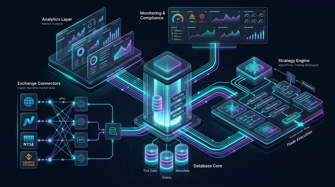Reference architecture: exchange connectors, columnar database core, analytics layer, strategy engine, and monitoring dashboards — all interconnected

Let's design a complete QuestDB-powered algorithmic trading platform for crypto markets. This architecture handles ingestion from multiple exchanges, real-time analytics, backtesting, and strategy execution.

Data Ingestion Layer

Data ingestion: multiple exchange connectors feed real-time market data through WebSocket pipelines into QuestDB via ILP

Multiple WebSocket connections to exchanges (Binance, Bybit, OKX, etc.) feed raw market data into QuestDB via ILP over HTTP. Each exchange connector is a separate process, providing isolation and fault tolerance.

Data streams include: trades (timestamp, symbol, side, price, quantity), order book snapshots (timestamp, symbol, bids[][], asks[][]), and funding rates/liquidations as auxiliary streams.

Ingestion throughput target: millions of rows per second across all exchanges combined. QuestDB's WAL handles this comfortably, with deduplication catching the inevitable duplicates from redundant exchange connections.

Real-Time Analytics Layer

Materialized views form the core of the analytics layer:

Raw trades → ohlc_1s → ohlc_5s → ohlc_1m → ohlc_5m → ohlc_15m → ohlc_1h → ohlc_1d

Each level refreshes incrementally. A Grafana dashboard connected via QuestDB's native plugin queries these views for candlestick charts, with sub-5ms response times regardless of how much historical data exists.

Additional materialized views compute: VWAP (volume-weighted average price) per symbol per day, rolling volatility estimates, and cross-exchange spread monitoring.

LATEST ON queries against pre-aggregated views power the real-time portfolio dashboard — showing current positions, unrealized P&L, and per-exchange exposure.

Strategy Engine

Strategy engine: real-time indicator computation feeds algorithmic decision-making, with buy/sell execution paths optimized by materialized views

Trading strategies query QuestDB for current market state and historical patterns. QuestDB's PG wire protocol means any language with a PostgreSQL driver can connect: Python for research strategies, Rust or C++ for latency-sensitive execution.

Key query patterns for strategies: ASOF JOIN for matching execution fills to market conditions at fill time, WINDOW JOIN for computing short-horizon metrics around each event, and window functions for real-time indicator computation (RSI, Bollinger Bands, ATR).

For latency-critical strategies, pre-computed materialized views minimize query time. A grid bot monitoring 50 symbols doesn't need to compute 50 separate moving averages on every tick — it reads them from a materialized view.

Backtesting Pipeline

Historical data lives in Parquet on object storage. QuestDB queries it transparently, but for heavy backtesting workloads, the data can also be read directly by Polars, Pandas, or DuckDB — bypassing the database entirely.

This dual-access pattern is powerful: live strategy uses QuestDB's SQL interface for real-time decisions, while the backtesting framework reads the same data through Parquet/Arrow for batch processing. Same data, two optimized access paths.

Monitoring and Post-Trade Analysis

HORIZON JOIN powers the post-trade analysis pipeline:

• Slippage analysis: Compare execution price to mid-price at fill time
• Markout curves: Track price evolution 1s, 5s, 30s, 60s after each fill
• Implementation shortfall: Decompose execution costs into spread, temporary impact, and permanent impact
• Venue scoring: Compare fill quality across exchanges to optimize order routing

These analyses run as scheduled queries, writing results to dedicated tables that feed monitoring dashboards. Alert rules trigger on anomalies — sudden slippage spikes, unusual markout patterns, or degraded fill quality on specific venues.

Performance Considerations

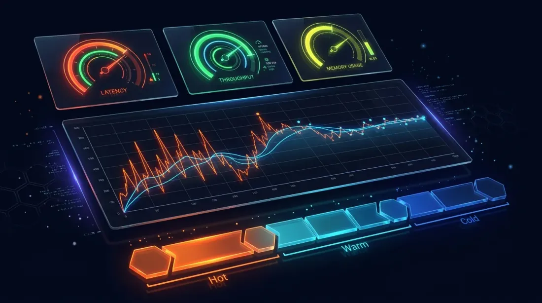Production performance tuning: latency, throughput, and memory monitoring alongside the hot-warm-cold data lifecycle

Some practical notes from production deployments:

Partition sizing: For crypto tick data with millions of rows per day, PARTITION BY HOUR is typically optimal. This keeps individual partitions manageable for both storage and query performance.

Materialized view cascading: Don't create too many intermediate levels. Each level adds refresh latency. For most use cases, 3-4 levels (1s → 1m → 15m → 1d) provide a good balance between query performance and data freshness.

Deduplication overhead: Enable deduplication on tables with redundant data sources. The cost is minimal for unique-timestamp data but increases with many same-timestamp rows that need column-level deduplication.

Memory allocation: QuestDB's zero-GC engine is efficient, but allocate enough memory for hot partitions and the write cache. Monitor via the built-in metrics endpoint.

Client protocol choice: Use ILP over HTTP for ingestion (with automatic retries and health checks). Use PG wire for queries. The ILP Protocol Version 2 (binary encoding) is significantly more efficient for array data and high-throughput double values.

QuestDB vs. The Alternatives

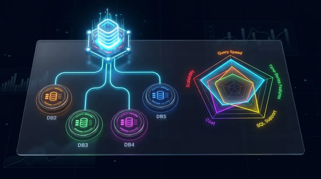Competitive landscape: QuestDB positioned against TimescaleDB, ClickHouse, InfluxDB, and kdb+ across key capability dimensions

A brief positioning against databases commonly used in trading:

vs. TimescaleDB: TimescaleDB is PostgreSQL with time-series extensions. It inherits PG's generality but also its overhead. QuestDB's native columnar engine and SIMD execution deliver significantly better query performance on time-series workloads, and features like ASOF JOIN have no direct TimescaleDB equivalent.

vs. ClickHouse: ClickHouse excels at analytical queries over massive datasets. But it wasn't designed for time-series specifically — no native ASOF JOIN, no SAMPLE BY with FILL, no 2D arrays for order books. For mixed OLAP + time-series workloads, ClickHouse might win; for pure trading data, QuestDB is more ergonomic.

vs. InfluxDB: InfluxDB has high-cardinality limitations that are painful for multi-exchange crypto data. Its query language (Flux, now deprecated; InfluxQL) lacks the expressiveness of QuestDB's SQL extensions. Performance on large historical queries is generally worse.

vs. kdb+/q: The gold standard for HFT. kdb+ is faster for certain single-threaded vector operations and its q language is incredibly concise. But it's proprietary, expensive, and has a steep learning curve. QuestDB offers 80-90% of the capability at a fraction of the cost, with standard SQL and open-source licensing.

Conclusion: A Database That Understands Trading

Over these three articles, we've covered QuestDB's architecture (three-tier storage with WAL, columnar, and Parquet), its SQL extensions (SAMPLE BY, ASOF JOIN, HORIZON JOIN, WINDOW JOIN, LATEST ON, TWAP), and its practical applications (materialized views, order book arrays, reference architecture).

The throughline is consistent: QuestDB was designed for exactly the workloads that algorithmic trading produces. It doesn't force you to work around the database — instead, its primitives map directly to trading concepts. OHLC aggregation is a one-liner. Trade-to-quote alignment is a single JOIN. Post-trade analysis is a HORIZON JOIN, not a multi-page PL/SQL procedure.

For teams building trading infrastructure — whether it's a crypto market data platform, a quantitative research environment, or a full algorithmic trading engine — QuestDB is worth serious evaluation. The open-source version covers most use cases, and the Enterprise edition fills the gaps for regulated environments.

The financial data infrastructure landscape is evolving rapidly. Databases that speak the language of markets will win. QuestDB is fluent.

Happy trading, and may your latencies be low.

Citation

@software{soloviov2025questdb_algotrading_p3,
  author = {Soloviov, Eugen},
  title = {QuestDB for Algorithmic Trading: From Order Books to Production Architecture},
  year = {2025},
  url = {https://marketmaker.cc/en/blog/post/questdb-algotrading-production},
  version = {0.1.0},
  description = {Materialized views, 2D array order book analytics, and reference architecture for a QuestDB-powered algorithmic trading platform.}
}