Neural ODEs: Does Continuous Time Beat a Delta-Time Feature?

Neural Ordinary Differential Equations (Chen et al., NeurIPS 2018) hidden state के derivative को neural network से parameterize करते हैं और output निकालने के लिए ODE solver को काम करने देते हैं। Model continuous-depth बन जाता है और, markets के लिए अधिक उपयोगी रूप से, continuous-time भी: hidden state को किसी भी पर evaluate किया जा सकता है, केवल उन grid points पर नहीं जहां आपका data संयोग से बैठता है।
इस property का financial data के लिए स्पष्ट pitch है, जो random intervals पर आता है। लेकिन यह pitch जितना दिखती है उससे कहीं कमजोर claim छिपाती है। एक साधारण GRU को अतिरिक्त input feature — पिछले observation के बाद से — दे दें, तो वह भी "जानता" है कि कितना समय बीता। असली सवाल यह नहीं है कि continuous-time models irregular data ले सकते हैं या नहीं। सवाल है कि क्या observations के बीच learned continuous dynamics ऐसी कोई चीज निकालती हैं जो delta-time feature पहले से नहीं देती, जबकि inference cost दस से सौ गुना हो।
यह लेख उस experiment को स्थापित करता है, इसे चलाने के लिए पूरा toolchain देता है और बताता है कि machinery को उचित ठहराने के लिए comparison को क्या दिखाना होगा। Bar construction वाला तर्क — कि trade timing स्वयं signal रखती है — beyond time bars में 17 bar types पर मापे गए evidence के साथ स्थापित है; यहां महत्वपूर्ण एकमात्र consequence modeling का है: solver hidden state को मनमाने पर evaluate करता है, इसलिए interpolation या padding की आवश्यकता नहीं।
परीक्षणाधीन दावा
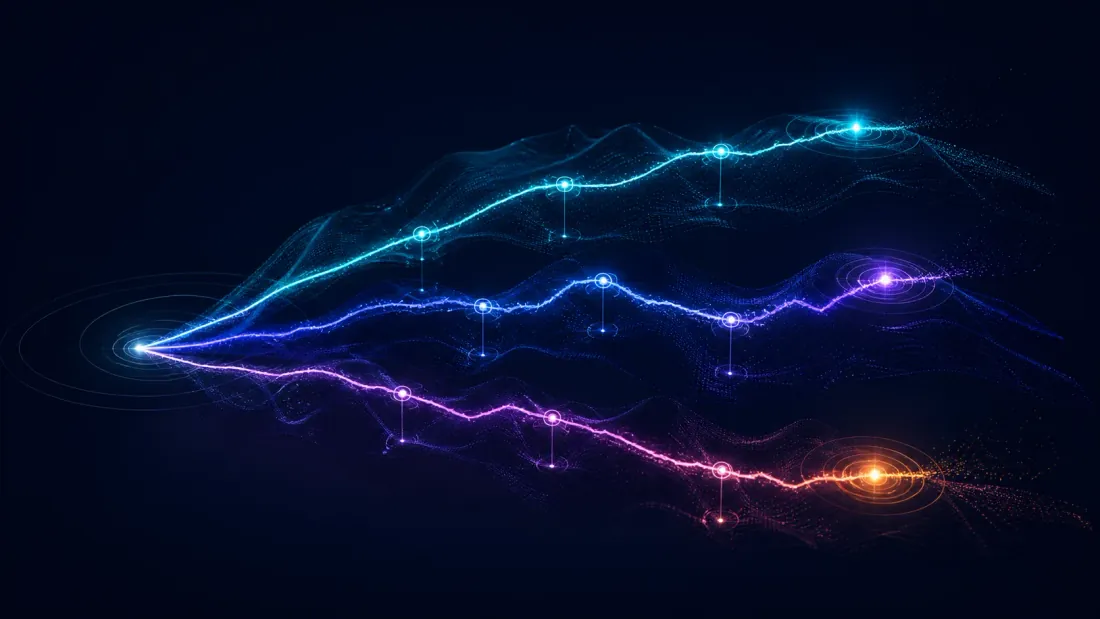
तीन nested hypotheses, जिनमें हर अगली पिछली से सख्त है:
- H1 — Raw irregular BTC trade stream पर fit किया गया ODE-RNN उसी stream पर बिना किसी time information के fit किए गए GRU से बेहतर है। यह लगभग निश्चित और लगभग बेकार है: ODE-RNN के पास वह information है जो baseline में नहीं है।
- H2 — जब GRU को input feature दिया जाए, तब भी ODE-RNN वही GRU हराता है। यही ईमानदार test है। Neural ODE literature को आम तौर पर यही claim करते हुए पढ़ा जाता है और financial data पर इसे लगभग कभी demonstrate नहीं किया गया।
- H3 — H2 का advantage latency budget के बाद भी बचा रहता है, अर्थात ODE-RNN live inference के लिए पर्याप्त तेज fixed-step solver के साथ भी यह advantage रखता है, adaptive
dopri5के साथ ही नहीं।
प्रयोग प्रोटोकॉल
दोनों arms के लिए वही tick stream, वही target और वही tuning budget। 1m bars पर resample न करें — resampling उस exact structure को नष्ट करता है जिसकी जांच हो रही है।
| सेटिंग | |
|---|---|
| डेटा | BTC trade prints, variable inter-arrival times, resampling नहीं |
| आर्म्स | ODE-RNN; GRU + ; बिना time feature वाला GRU |
| लक्ष्य | सभी आर्म्स के लिए समान; fit के साथ निर्दिष्ट |
| मेट्रिक्स | RMSE, held-out log-likelihood, प्रति epoch wall-clock, प्रति step inference latency |
| Solver sweep | dopri5 (rtol 1e-5) बनाम fixed-step Euler, training accuracy पर matched |
| विभाजन | Walk-forward, केवल out-of-sample |
| आर्म | RMSE | Log-lik | s/epoch | प्रति step inference latency |
|---|---|---|---|---|
| GRU (no time feature) | — | — | — | — |
| GRU + log(dt) | — | — | — | — |
| ODE-RNN (dopri5) | — | — | — | — |
| ODE-RNN (fixed-step Euler) | — | — | — | — |
H2 पर negative result पूरी तरह publishable है और संभवतः अधिक मूल्यवान outcome भी — यही standard ईमानदार negative result और multiple testing के तहत deflated Sharpe में लागू किया गया है।
द्वितीयक प्रयोग: CNF बनाम Student-t
यदि ODE-RNN comparison बहुत महंगा हो, तो सस्ता empirical anchor distributional है: real BTC daily returns पर continuous normalizing flow fit करें और उसकी fitted density की तुलना Student-t fit तथा empirical tail से करें, और 1% तथा 5% levels पर tail-quantile errors report करें। यह सीधे उस distributional work से जुड़ता है जिसे GARCH volatility forecasting और asymmetric GARCH में पहले मापा गया है।
इस लेख का बाकी हिस्सा ऊपर के experiment को चलाने के लिए जरूरी background और toolchain है।
पृष्ठभूमि: ResNets से continuous dynamics तक

Residual network compute करता है। Step size घटाएं और layers की संख्या बढ़ाएं, तो continuous limit के करीब पहुंचते हैं:
अलग-अलग parameters वाली discrete layers के बजाय एक single network instantaneous rate of change को specify करता है। Time पर output initial value problem को solve करता है:
Black-box solver (Euler, Runge-Kutta, Dormand-Prince) integral को numerically compute करता है और local error estimates से step sizes adaptively चुनता है।
Adjoint method
हर solver step के through backpropagate करने पर सभी intermediate states store करने पड़ते हैं, जिसकी memory step count के proportional होती है। Chen et al. इसके बजाय memory के साथ backward ODE solve करते हैं। Adjoint state परिभाषित करें, जो satisfy करता है
और backward pass के दौरान parameter gradient accumulate करें:
Backward pass एक augmented system solve करता है जो , और को एक साथ compute करता है, और solver को से तक उल्टी दिशा में चलाता है।
Trade-off यह है: को पीछे की ओर reconstruct करने पर numerical error accumulate होता है, खासकर stiff या chaotic dynamics के लिए। Checkpointing बीच का रास्ता है — कुछ intermediate times पर store करें और उनके बीच recompute करें। Price processes continuous semimartingales और moderately smooth होते हैं, इसलिए adjoint आम तौर पर ठीक रहता है; microstructure events के आसपास stiffness adaptive solvers या hybrids को मजबूर कर सकती है।
ODE-RNN: Observations के बीच continuous hidden state

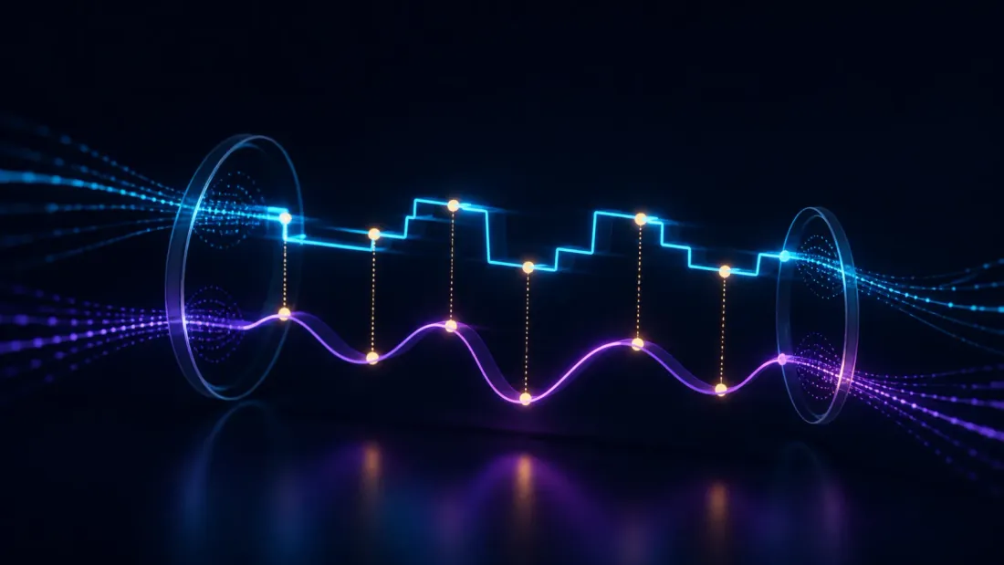
ODE-RNN वह architecture है जिस पर मुख्य experiment निर्भर करता है। Observations के बीच hidden state ODE के अंतर्गत evolve होता है:
जब observation समय पर आता है, तब discrete update fire होता है:
Superscripts observation के ठीक पहले और बाद की state को दर्शाते हैं। Observations के बीच learned continuous dynamics; observations पर नई information।
H2 ablation जिस mechanism को probe करती है वह यह है: लंबा gap होने पर hidden state के तहत लंबी दूरी तक evolve हुई है — baseline की ओर decay करते हुए या diverge करते हुए — और उस evolution का shape सीखा गया है, scalar के रूप में दिया नहीं गया। Real trade data पर यह expressiveness अपनी लागत चुकाती है या नहीं, यही अभी unmeasured है।
Ticks से आगे के natural fits: multi-asset portfolios जहां हर asset का अपना observation schedule हो और correlated assets की latent state evolve होती रहे जबकि केवल एक observe हो; तथा event-driven signals (news, earnings, macro releases) जो irregular times पर आते हैं।
Neural SDEs: Stochastic components जोड़ना

Neural ODEs deterministic हैं और price path में noise को represent नहीं कर सकते। Classical treatment — geometric Brownian motion, risk-neutral drift और constant-volatility assumptions के smile के विरुद्ध fail होने के तरीके — Black-Scholes options pricing में cover है। Neural SDEs parametric form को learned diffusion term से बदलते हैं:
drift है, diffusion, Wiener process; और दोनों neural networks हैं।
Architecture: Drift Net और Diffusion Net
- Drift net : expected trajectory — trend, mean reversion, momentum। Prediction error को minimize करने के लिए train किया जाता है।
- Diffusion net : noise magnitude, state के function के रूप में सीखा जाता है। Volatile regimes में अधिक, calm regimes में कम।
यह split classical quant finance को mirror करता है: drift risk-neutral (या P-measure) dynamics है, diffusion volatility surface है।
Neural SDEs का training
Stochastic integral classical sense में differentiable नहीं है। तीन approaches हैं:
- Pathwise gradients: reparameterization trick — Brownian paths sample करें और noise को fixed input मानकर solver के through differentiate करें।
- Score matching: estimate करें और denoising objectives के माध्यम से train करें — यही machinery crypto prediction के लिए diffusion models में standalone generative model के रूप में इस्तेमाल होती है; यहां इसे SDE के training option तक सीमित किया गया है।
- Finite-dimensional distribution matching: full path measures के बजाय observation times पर marginals match करें।
Pathwise practical default है। torchsde autodiff support के साथ Euler-Maruyama, Milstein और stochastic Runge-Kutta implement करता है।
Volatility surface सीखना
Classical models (Heston, SABR) diffusion coefficient पर parametric forms impose करते हैं। Neural SDE को arbitrary function के रूप में सीखता है:
यह diffusion processes के लिए universal approximator है — पर्याप्त capacity मिलने पर कोई भी Ito process arbitrary accuracy तक।
Missing और asynchronous data के लिए Latent ODEs

Latent ODE (Rubanova, Chen, Duvenaud, 2019) Neural ODE को VAE के साथ जोड़ता है: financial series smooth underlying process की noisy observations हैं, जिसे low-dimensional latent space में सीखा जाता है।
- Recognition network: observations के through backward चलने वाला ODE-RNN, जो produce करता है।
- Latent dynamics: ।
- Decoder: , किसी भी requested time पर evaluate किया जा सकता है।
Loss standard ELBO है:
Portfolio state estimation: assets के बीच sparse asynchronous observations से joint dynamics को capture करने वाली continuous latent state infer करें — मूलतः Kalman filter का nonlinear, learned version।
Missing data imputation: halts और weekend gaps को smoothly interpolated latent trajectory मिलती है; decoder VAE posterior की uncertainty के साथ gap के through plausible paths produce करता है।
Multi-frequency fusion: daily closes, intraday VWAP और tick data एक ही model में, shared time grid के बिना।
Return distributions के लिए Continuous Normalizing Flows
CNFs simple base distribution को complex target में बदलने के लिए Neural ODE का उपयोग करते हैं। Transformation है और log-density instantaneous change of variables का पालन करती है:
State और log-density को से आगे integrate करें ताकि और मिलें। Scalability के लिए Jacobian trace को Hutchinson stochastic estimator से estimate किया जाता है।
Crypto returns leptokurtic और negatively skewed हैं — real data पर GARCH volatility forecasting और asymmetric GARCH तथा leverage effect में मापे गए — और CNF उस shape को assume करने के बजाय सीखता है। Flow को state variables पर condition करने से shape regime के साथ बदल सकती है। Density exact है, approximate नहीं, इसलिए यह Monte Carlo और bootstrap backtests में compute किए गए tail metrics और HRP/CVaR portfolio pipeline के CVaR construction को feed कर सकती है; joint tail structure को joint risk के लिए copula models में अलग संभाला गया है।
Conditional density estimation
Useful framing एक ही problem के तीन published approaches का सीधा contrast है। TFT quantile output layer से fixed quantiles का set देता है। Conformal prediction coverage guarantee वाले calibrated intervals देता है। Conditional CNF exact, differentiable density देता है:
Differentiability distinguishing property है: density downstream objective के भीतर बैठ सकती है और उसके through backpropagate की जा सकती है, जिसे fixed quantiles या conformal intervals support नहीं करते। उसी target पर TFT quantiles के विरुद्ध exact density की लागत उचित है या नहीं, यहां untested है।
Discrete alternatives से तुलना
| गुण | LSTM/GRU | Transformer | Neural ODE | Neural SDE |
|---|---|---|---|---|
| अनियमित समय प्रबंधन | कमजोर (padding चाहिए) | Positional encoding | Native | Native |
| Memory (training) | adjoint | adjoint | ||
| Uncertainty quantification | नहीं (deterministic) | नहीं (deterministic) | ensembles से | Native |
| Observations के बीच interpolation | नहीं | नहीं | हां | हां |
| Continuous-time density | नहीं | नहीं | CNF से | path measure से |
| Computational cost | कम | मध्यम | Variable (solver) | अधिक (SDE solver) |
इस table का LSTM-versus-attention आधा भाग benchmarks के साथ TFT article में detail में argument किया गया है — उसके "TFT vs LSTM vs Vanilla Transformer" और "When LSTM Still Wins" sections देखें। यहां नए columns दाईं ओर के दो हैं, और H2/H3 questions का निर्णय करने वाली rows अंतिम दो हैं।
torchdiffeq के साथ Python implementation

torchdiffeq adjoint backpropagation के साथ ODE solvers provide करता है।
Price dynamics के लिए Basic Neural ODE
import torch
import torch.nn as nn
from torchdiffeq import odeint_adjoint as odeint

class PriceDynamics(nn.Module):
    """Neural network defining dh/dt = f(h, t)."""

    def __init__(self, hidden_dim: int = 64):
        super().__init__()
        self.net = nn.Sequential(
            nn.Linear(hidden_dim, 128),
            nn.Tanh(),
            nn.Linear(128, 128),
            nn.Tanh(),
            nn.Linear(128, hidden_dim),
        )

    def forward(self, t, h):
        return self.net(h)


class NeuralODEPredictor(nn.Module):
    """
    Encode observed features -> latent state,
    evolve via Neural ODE,
    decode to price prediction.
    """

    def __init__(self, input_dim: int, hidden_dim: int = 64):
        super().__init__()
        self.encoder = nn.Linear(input_dim, hidden_dim)
        self.dynamics = PriceDynamics(hidden_dim)
        self.decoder = nn.Linear(hidden_dim, 1)

    def forward(self, x0, eval_times):
        """
        x0:         (batch, input_dim) features at t=0
        eval_times: (T,) times at which to evaluate the ODE
        Returns:    (T, batch, 1) predictions
        """
        h0 = self.encoder(x0)                          # (batch, hidden_dim)
        h_traj = odeint(self.dynamics, h0, eval_times,
                        method='dopri5', rtol=1e-5, atol=1e-7)
        return self.decoder(h_traj)
अनियमित tick data के लिए ODE-RNN
यह experimental arm है। इसे हराना जरूरी baseline उसी stream पर nn.GRUCell है, जिसमें log(t_next - t_prev) को x के साथ concatenate किया गया है।
class ODERNNCell(nn.Module):
    """Single step: ODE-evolve, then RNN-update."""

    def __init__(self, input_dim: int, hidden_dim: int = 64):
        super().__init__()
        self.dynamics = PriceDynamics(hidden_dim)
        self.gru_cell = nn.GRUCell(input_dim, hidden_dim)

    def forward(self, h, x, t_prev, t_next):
        times = torch.tensor([t_prev, t_next], dtype=torch.float32)
        h_evolved = odeint(self.dynamics, h, times,
                           method='dopri5')[-1]  # state at t_next
        h_updated = self.gru_cell(x, h_evolved)
        return h_updated


class ODERNN(nn.Module):
    """Process irregularly-sampled sequence."""

    def __init__(self, input_dim: int, hidden_dim: int = 64):
        super().__init__()
        self.cell = ODERNNCell(input_dim, hidden_dim)
        self.decoder = nn.Linear(hidden_dim, 1)
        self.hidden_dim = hidden_dim

    def forward(self, observations, times):
        """
        observations: list of (batch, input_dim) tensors
        times:        list of floats, observation timestamps
        """
        batch_size = observations[0].shape[0]
        h = torch.zeros(batch_size, self.hidden_dim)

        outputs = []
        for i in range(len(observations)):
            t_prev = 0.0 if i == 0 else times[i - 1]
            h = self.cell(h, observations[i], t_prev, times[i])
            outputs.append(self.decoder(h))

        return torch.stack(outputs)  # (seq_len, batch, 1)
Training loop
def train_neural_ode(model, train_loader, epochs=100, lr=1e-3):
    optimizer = torch.optim.Adam(model.parameters(), lr=lr)
    scheduler = torch.optim.lr_scheduler.CosineAnnealingLR(
        optimizer, T_max=epochs
    )

    for epoch in range(epochs):
        epoch_loss = 0.0
        for batch in train_loader:
            features, times, targets = batch
            optimizer.zero_grad()

            predictions = model(features, times)
            loss = torch.nn.functional.mse_loss(predictions, targets)

            loss.backward()
            torch.nn.utils.clip_grad_norm_(model.parameters(), max_norm=1.0)
            optimizer.step()

            epoch_loss += loss.item()

        scheduler.step()

        if (epoch + 1) % 10 == 0:
            avg_loss = epoch_loss / len(train_loader)
            print(f"Epoch {epoch+1}/{epochs}, Loss: {avg_loss:.6f}")
Return distributions के लिए Continuous Normalizing Flow
from torchdiffeq import odeint

class CNFDynamics(nn.Module):
    """Dynamics for continuous normalizing flow."""

    def __init__(self, dim: int = 1, hidden_dim: int = 64):
        super().__init__()
        self.net = nn.Sequential(
            nn.Linear(dim + 1, hidden_dim),  # +1 for time
            nn.Tanh(),
            nn.Linear(hidden_dim, hidden_dim),
            nn.Tanh(),
            nn.Linear(hidden_dim, dim),
        )
        self.dim = dim

    def forward(self, t, state):
        z = state[..., :self.dim]
        t_expand = t.expand(z.shape[0], 1)
        zt = torch.cat([z, t_expand], dim=-1)
        dz = self.net(zt)

        e = torch.randn_like(z)
        e_dz = torch.autograd.grad(
            dz, z, e, create_graph=True
        )[0]
        trace_jac = (e_dz * e).sum(dim=-1, keepdim=True)

        return torch.cat([dz, -trace_jac], dim=-1)


class ReturnDistributionCNF(nn.Module):
    """Model return distributions with continuous normalizing flows."""

    def __init__(self, dim: int = 1):
        super().__init__()
        self.dynamics = CNFDynamics(dim)
        self.dim = dim

    def log_prob(self, x):
        """Compute log probability of observed returns."""
        log_p0 = torch.zeros(x.shape[0], 1)
        state0 = torch.cat([x, log_p0], dim=-1)
        state0.requires_grad_(True)

        times = torch.tensor([1.0, 0.0])  # backward
        state_T = odeint(self.dynamics, state0, times,
                         method='dopri5')[-1]

        z_T = state_T[..., :self.dim]
        delta_log_p = state_T[..., self.dim:]

        log_p_base = -0.5 * (z_T ** 2 + torch.log(
            torch.tensor(2 * torch.pi)
        )).sum(dim=-1, keepdim=True)

        return log_p_base + delta_log_p

    def sample(self, n_samples: int):
        """Generate samples from learned distribution."""
        z0 = torch.randn(n_samples, self.dim)
        log_p0 = torch.zeros(n_samples, 1)
        state0 = torch.cat([z0, log_p0], dim=-1)

        times = torch.tensor([0.0, 1.0])  # forward
        state_T = odeint(self.dynamics, state0, times,
                         method='dopri5')[-1]

        return state_T[..., :self.dim]
व्यावहारिक नोट्स

ऊपर के experiment को चलाते समय यही चीजें आपको परेशान करेंगी।
Solver choice और speed
dopri5 accuracy guarantees देता है लेकिन compute cost variable है, इसलिए H3 H2 से अलग hypothesis है: adaptive solver के तहत मौजूद edge live latency budget में survive नहीं कर सकता। Fixed-step solvers (Euler, RK4) accuracy की कीमत पर predictable latency देते हैं। Practical compromise: dopri5 के साथ train करें, fixed-step solver के साथ deploy करें जिसे representative data पर adaptive solver के output से match करने के लिए calibrate किया गया हो — और gap को छोटा मानने के बजाय मापें।
odeint(f, h0, t, method='dopri5', rtol=1e-6, atol=1e-8)

odeint(f, h0, t, method='euler', options={'step_size': 0.1})
Discontinuous jumps के पास stiff problems के लिए method='implicit_adams' या method='scipy_solver'।
Numerical stability
यदि बड़े values output करता है, तो state diverge करती है। Mitigations:
- की layers पर Spectral normalization, ताकि Lipschitz constant नियंत्रित रहे।
- Training के दौरान Gradient clipping (ऊपर training loop में दिखाया गया)।
- Time normalization: timestamps को में scale करें।
- Dynamics norm पर regularization: loss में जोड़ें।
Integration interval
कई महीनों तक फैले data के लिए से minutes तक integrate न करें:
t_normalized = (timestamps - timestamps[0]) / (timestamps[-1] - timestamps[0])
यह solver को numerically friendly regime में रखता है और learned dynamics को scale-invariant बनाता है। Comparison के लिए भी यह महत्वपूर्ण है: unnormalized ODE-RNN केवल numerical कारणों से GRU baseline से हार सकता है, जो finding के बजाय measurement artifact होगा।
Multiple time scales संभालना
Markets में microsecond, second, minute और daily scales की dynamics एक साथ होती हैं, और single Neural ODE को सभी को संभालना कठिन हो सकता है। Options: अलग-अलग time scales पर multiple ODE blocks stack करें; fast और slow दोनों capacity के लिए hidden dimension बढ़ाएं; या प्रति frequency band अलग Neural ODEs चलाकर outputs fuse करें। (यह model-capacity का सवाल है, adaptive resolution drill-down में backtest-fidelity के सवाल से अलग।)
खुले अनुसंधान निर्देश

Neural Jump SDEs: अचानक dislocations (flash crashes, earnings surprises) के लिए learned jump component जोड़ें:
जहां compensated Poisson random measure है और learned jump kernel है।
Neural Controlled Differential Equations (Neural CDEs): Wiener process को general driving signal से बदलें, ताकि observed data streams dynamics को drive करें। Order flow के लिए natural है, जहां trades और quotes का stream latent market state को drive करता है।
Differentiable Market Simulation: Neural SDE को differentiable simulator के भीतर generative model के रूप में इस्तेमाल करें और adjoint के माध्यम से backpropagate करके strategies को end-to-end train करें। Strategy और market model साथ-साथ evolve होते हैं।
Physics-Informed Neural ODEs: PINNs loss में differential-equation residual embed करते हैं — technique स्वयं Navier-Stokes article में introduce की गई है। Financial application यह है कि learned dynamics पर no-arbitrage, put-call parity और martingale conditions को penalty terms या hard constraints के रूप में impose किया जाए।
निष्कर्ष

Continuous-time framing structural रूप से सही है: markets continuous processes हैं जिन्हें discrete, irregular times पर observe किया जाता है, और models को इसका सम्मान करना चाहिए। Toolchain mature है — torchdiffeq, torchsde, बाकी के लिए plain PyTorch — और ज्ञात costs long integration intervals पर solver speed तथा numerical stability हैं।
जो स्थापित नहीं है, वह वह हिस्सा है जो तय करेगा कि इनमें से कुछ production stack में होना चाहिए या नहीं। Structural correctness predictive advantage का evidence नहीं है, और feature पर continuous dynamics के लिए दावा किया गया specific advantage यहां real trade data पर मापा नहीं गया है। जब तक ऊपर की H2 table भरी नहीं जाती, fold के नीचे के सभी अंशों को working implementation से जुड़ी well-specified hypothesis समझें, result नहीं।
संदर्भ
- Chen, R.T.Q., Rubanova, Y., Bettencourt, J., Duvenaud, D. (2018). Neural Ordinary Differential Equations. NeurIPS 2018. arXiv:1806.07366
- Rubanova, Y., Chen, R.T.Q., Duvenaud, D. (2019). Latent ODEs for Irregularly-Sampled Time Series. NeurIPS 2019. arXiv:1907.03907
- Jia, J., Benson, A.R. (2019). Neural Jump Stochastic Differential Equations. NeurIPS 2019.
- Kidger, P., Morrill, J., Foster, J., Lyons, T. (2020). Neural Controlled Differential Equations for Irregular Time Series. NeurIPS 2020.
- Hasan, A., Pereira, J.M., Farsiu, S., Carin, L. (2021). Neural Network Stochastic Differential Equation Models with Applications to Financial Data Forecasting. arXiv:2111.13164
- torchdiffeq: github.com/rtqichen/torchdiffeq
- UvA Deep Learning Tutorials — Neural ODEs: uvadlc-notebooks.readthedocs.io
Authors
Trading-systems engineer
Trading-systems engineer building bots since 2017: cross-exchange arbitrage (connected up to 30 venues), cointegration-based pairs arbitrage across spot and futures, scalping, news and sentiment-driven strategies, trend algorithms, and portfolio management and balancing algorithms. Also builds sub-millisecond order execution, big-data warehouses, backtesting engines, AI agents, and trading interfaces (incl. open-source profitmaker.cc). Stack: JS/TS, Python, Rust/Zig/Go, DevOps, backend, frontend, architecture.
Read More

Hamiltonian Neural Networks: Does a Financial System Conserve Anything?

Trade Classification When You Have No Side Flag: Tick, Quote, Lee-Ready, BVC