シグナル相関:何ペア監視すべきか

10個の暗号通貨ペアで戦略を立ち上げます:BTC/USDT、ETH/USDT、SOL/USDT、AVAX/USDTなど。ロジックは完璧に見えます:1ペアで戦略がアクティブな時間が5%なら、10ペアでは少なくとも1つがアクティブである時間は。稼働率が4倍になるはずです。
実際には、稼働率は40%ではなく15-16%です。10ペアが3ペアのように振る舞います。資本は遊休し、fill_efficiencyは低下し、実効ポートフォリオリターンは予測の3分の1になります。
原因はシグナル相関です。そして暗号通貨では、それは壊滅的に高いのです。
暗号通貨における分散の幻想

伝統的な金融では、Apple株と石油ETFが異なる要因に反応するため、分散が機能します。暗号通貨市場では、すべてが異なります。
BTCが支配的な要因です。ビットコインが5%下落すると、ETHは6-8%下落し、SOLは8-12%下落し、アルトコインは10-20%下落します。暗号通貨市場における日次リターンの相関は一貫して0.6を超え、パニック時には1.0に近づきます。
しかし、アルゴトレーダーである私たちにとって重要なのは、価格の相関ではなくシグナルの相関です。戦略がモメンタムに基づいていて、BTCがエントリーシグナルをトリガーした場合、ETHとSOLも同じ分以内に類似のシグナルをトリガーする確率が高いです。すべてのペアが同時にロングに入り、同時に退出します。10ポジション — しかし本質的には1つの賭けです。
なぜ10ペア ≠ 10倍の分散なのか

形式的な定式化
各ペアで戦略が時間の割合アクティブであるとします。シグナルが完全に独立であれば、少なくとも1ペアがアクティブである確率:
戦略B(、)の場合:
しかし、シグナルは独立ではありません。暗号通貨は同期して動きます — つまり、シグナルはクラスターで発生し消滅します。
相関が10ペアを3ペアに変える
直感はこうです:10ペアが相関している場合、10の独立したソースではなく、3-4のソースからの情報を持っています。これをeffective_Nを通じて形式化します:
ここではcorrelation factorであり、平均ペアワイズシグナル相関を反映します。のときペアは完全に独立、のとき同一です。
暗号通貨ペアの場合、典型的な。すると:
40%ではなく15.6%。2.5倍の差です。Fill efficiencyもそれに応じて低下し、ポートフォリオ全体の実効リターンも低下します(PnL per Active Timeを参照)。
暗号通貨市場における相関

支配的要因としてのBTC
暗号通貨市場は顕著なファクター構造を持っています。BTCはほとんどのアルトコインの日次リターン分散の60-80%を説明します。これはPCA(主成分分析)を通じて明確に見ることができます:
import numpy as np
from sklearn.decomposition import PCA

def analyze_crypto_factor_structure(returns_matrix: np.ndarray, pair_names: list) -> dict:
    """
    PCA analysis of the factor structure of crypto returns.

    Args:
        returns_matrix: returns matrix [n_days x n_pairs]
        pair_names: list of pair names
    """
    pca = PCA()
    pca.fit(returns_matrix)

    explained = pca.explained_variance_ratio_
    cumulative = np.cumsum(explained)

    print("Factor structure:")
    for i, (var, cum) in enumerate(zip(explained[:5], cumulative[:5])):
        print(f"  PC{i+1}: {var:.1%} variance (cumulative: {cum:.1%})")

    loadings = pca.components_[0]
    print("\nPC1 loadings (BTC factor):")
    for name, load in sorted(zip(pair_names, loadings), key=lambda x: -abs(x[1])):
        print(f"  {name}: {load:.3f}")

    return {
        "explained_variance": explained,
        "n_effective_factors": int(np.searchsorted(cumulative, 0.90)) + 1,
        "pc1_loadings": dict(zip(pair_names, loadings)),
    }
10個の暗号通貨ペアのポートフォリオの典型的な結果:
| コンポーネント | 説明分散 | 累積 |
|---|---|---|
| PC1 (BTC) | 65% | 65% |
| PC2 | 12% | 77% |
| PC3 | 8% | 85% |
| PC4 | 5% | 90% |
| PC5-PC10 | 10% | 100% |
4つのファクターが分散の90%を説明します。10ペアのうち、「独立」しているのは最大4つです。
シグナル相関と価格相関の違い
重要なニュアンスがあります。価格の相関とシグナルの相関は異なるものです。BTCとETHの価格相関は0.85ですが、特定の戦略のシグナル相関はエントリーロジックに応じて0.95にも0.50にもなり得ます。
例:RSIの買われすぎ/売られすぎ戦略。BTCのRSIが30を下回る(売られすぎ)— ロングでエントリー。ETHも同じ瞬間に売られすぎかもしれません(シグナル相関0.90)。あるいは、ETHがより緩やかに下落していた場合、そうでないかもしれません(シグナル相関0.40)。
正しいアプローチは、価格系列ではなく、シグナルそのものの相関を測定することです:
import numpy as np
from itertools import combinations

def signal_correlation_matrix(
    signals: dict,  # {pair: np.array of 0/1 per minute}
    method: str = "pearson",
) -> np.ndarray:
    """
    Calculate the signal correlation matrix (binary: 0 = flat, 1 = in position).

    Args:
        signals: dictionary {pair_name: binary_signal_array}
        method: correlation method ("pearson", "jaccard")
    """
    pairs = sorted(signals.keys())
    n = len(pairs)
    corr_matrix = np.ones((n, n))

    for i, j in combinations(range(n), 2):
        s_i = signals[pairs[i]]
        s_j = signals[pairs[j]]

        if method == "pearson":
            corr = np.corrcoef(s_i, s_j)[0, 1]
        elif method == "jaccard":
            intersection = np.sum(s_i & s_j)
            union = np.sum(s_i | s_j)
            corr = intersection / union if union > 0 else 0
        else:
            raise ValueError(f"Unknown method: {method}")

        corr_matrix[i, j] = corr
        corr_matrix[j, i] = corr

    return corr_matrix, pairs


def estimate_correlation_factor(corr_matrix: np.ndarray) -> float:
    """
    Estimate correlation_factor from the signal correlation matrix.

    correlation_factor = 1 + (N-1) * mean_pairwise_correlation

    When correlation is 0 → C_f = 1 (all independent).
    When correlation is 1 → C_f = N (all identical).
    """
    n = corr_matrix.shape[0]
    upper_triangle = corr_matrix[np.triu_indices(n, k=1)]
    mean_corr = np.mean(upper_triangle)

    correlation_factor = 1 + (n - 1) * mean_corr
    return correlation_factor
時間的相関:平常時 vs. パニック時
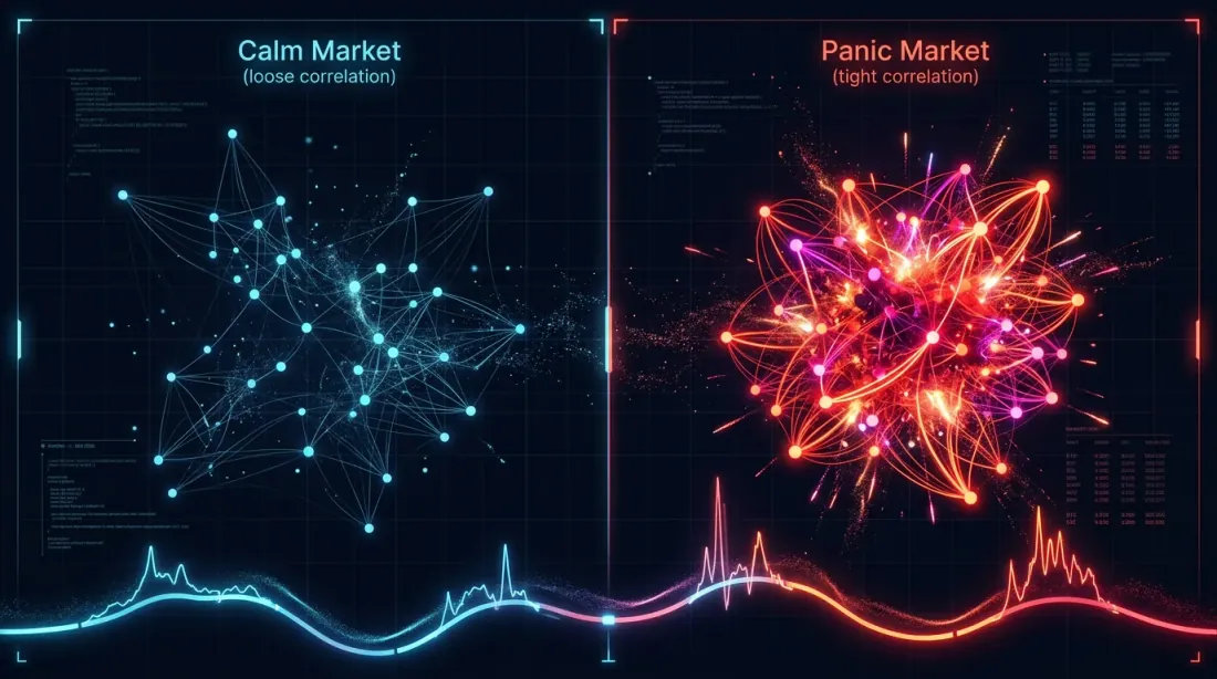
相関は静的ではありません。平常期間中、BTCとアルトコインは乖離する可能性があります — ETHはイーサリアムのニュースで上昇し、SOLはソラナのニュースで上昇します。危機時には、すべてが単一のファクターに崩壊します:リスクオン/リスクオフ。
def rolling_correlation_factor(
    signals: dict,
    window_days: int = 30,
    step_days: int = 7,
) -> list:
    """
    Rolling correlation_factor to detect regime changes.
    """
    pairs = sorted(signals.keys())
    minutes_per_day = 1440
    window = window_days * minutes_per_day
    step = step_days * minutes_per_day

    total_minutes = len(signals[pairs[0]])
    results = []

    for start in range(0, total_minutes - window, step):
        end = start + window
        window_signals = {p: signals[p][start:end] for p in pairs}

        corr_matrix, _ = signal_correlation_matrix(window_signals)
        cf = estimate_correlation_factor(corr_matrix)

        results.append({
            "start_minute": start,
            "end_minute": end,
            "correlation_factor": cf,
            "effective_n": len(pairs) / cf,
        })

    return results
10個の暗号通貨ペアの典型的な様相:
| 市場レジーム | 平均シグナル相関 | ||
|---|---|---|---|
| レンジ相場(低ボラティリティ) | 0.15-0.25 | 2.4-3.3 | 3.0-4.2 |
| 上昇トレンド | 0.25-0.40 | 3.3-4.6 | 2.2-3.0 |
| 下降トレンド | 0.30-0.50 | 3.7-5.5 | 1.8-2.7 |
| パニック(暴落) | 0.60-0.90 | 6.4-9.1 | 1.1-1.6 |
パニック時には、10ペアが1-2の実効ペアに圧縮されます。分散が最も必要なときに、それが消失するのです。これは古典的な「危機時には相関が1に向かう」の暗号通貨版です。
effective_N:核心概念

公式と導出
effective_Nのアイデアは統計学から借用したもので、有効標本サイズが観測値の自己相関を考慮するものです。我々の目的では:
ここでは平均ペアワイズシグナル相関です。簡略表記:
性質:
- のとき:、 — 完全独立
- のとき:、 — すべてのペアが同一
- かつのとき:、
データからcorrelation_factorを推定する方法
実践では3つのアプローチがあります:
1. シグナル相関行列から(正確)。
すべてのペアで戦略を実行し、バイナリシグナル(各分ごとの0/1)を取得し、相関行列を構築し、上記の公式を使ってを計算します。
2. 価格リターンのPCAから(近似)。
シグナルが価格ダイナミクス(モメンタム、平均回帰)に強く依存する場合、を分散の90%を説明するPCAコンポーネント数として推定できます。
3. 資産クラスのヒューリスティクスから(概算)。
| 資産クラス | 典型的な |
|---|---|
| 暗号通貨(トップ10) | 2.5-4.0 |
| 暗号通貨(DeFi/ミームコイン含む) | 2.0-3.0 |
| 外国為替(メジャー) | 1.5-2.5 |
| 株式(単一セクター) | 2.0-3.5 |
| 株式(クロスセクター) | 1.2-1.8 |
BTC、ETH、SOL、AVAX、MATIC、DOGE、DOT、LINK、UNI、ATOMの暗号通貨ポートフォリオの場合、安全な推定値はです。
スロット稼働率モデリング

の公式
相関を考慮した基本公式:
異なる戦略とペア数の表():
| 戦略 | (取引時間) | 5ペア() | 10ペア() | 20ペア() | 50ペア() |
|---|---|---|---|---|---|
| 戦略B | 5% | 8.2% | 15.6% | 29.1% | 58.0% |
| 戦略A | 15% | 23.6% | 41.8% | 65.9% | 92.8% |
| 戦略C | 45% | 67.1% | 89.0% | 98.8% | ~100% |
5%のアクティビティの戦略Bでは、少なくとも1つのアクティブポジションが半分の時間ある状態にするために50ペアが必要です。しかも、50の暗号通貨ペアは10より強く相関しているという事実を考慮していません。
マルチスロットオーケストレーター
実際のオーケストレーターは複数のスロットを同時に管理します。5スロットと10ペアがある場合、稼働率の計算は異なります:
def estimate_fill_efficiency(
    trading_time_pct: float,
    n_pairs: int,
    correlation_factor: float = 3.0,
    max_slots: int = 1,
) -> dict:
    """
    Analytical estimate of fill efficiency for a multi-slot orchestrator.

    Args:
        trading_time_pct: fraction of active time for one strategy on one pair
        n_pairs: number of trading pairs
        correlation_factor: signal correlation coefficient
        max_slots: maximum number of simultaneous positions

    Returns:
        dict with utilization metrics
    """
    effective_n = n_pairs / correlation_factor

    p_at_least_one = 1 - (1 - trading_time_pct) ** effective_n

    expected_active = effective_n * trading_time_pct

    utilization = min(expected_active, max_slots) / max_slots

    fill_efficiency = min(p_at_least_one, utilization)

    return {
        "effective_n": effective_n,
        "p_at_least_one": p_at_least_one,
        "expected_active": expected_active,
        "utilization": utilization,
        "fill_efficiency": fill_efficiency,
    }


configs = [
    ("Strategy B, 10 pairs, 1 slot", 0.05, 10, 3.0, 1),
    ("Strategy B, 10 pairs, 3 slots", 0.05, 10, 3.0, 3),
    ("Strategy B, 30 pairs, 1 slot", 0.05, 30, 3.0, 1),
    ("Strategy A, 10 pairs, 1 slot", 0.15, 10, 3.0, 1),
    ("Strategy C, 10 pairs, 1 slot", 0.45, 10, 3.0, 1),
    ("Strategy C, 10 pairs, 5 slots", 0.45, 10, 3.0, 5),
]

for name, p, n, cf, slots in configs:
    result = estimate_fill_efficiency(p, n, cf, slots)
    print(f"{name}:")
    print(f"  N_eff = {result['effective_n']:.1f}")
    print(f"  P(≥1 active) = {result['p_at_least_one']:.1%}")
    print(f"  E[active] = {result['expected_active']:.2f}")
    print(f"  fill_efficiency = {result['fill_efficiency']:.1%}")
    print()
期待される出力:
Strategy B, 10 pairs, 1 slot:
  N_eff = 3.3
  P(≥1 active) = 15.6%
  E[active] = 0.17
  fill_efficiency = 15.6%

Strategy B, 10 pairs, 3 slots:
  N_eff = 3.3
  P(≥1 active) = 15.6%
  E[active] = 0.17
  fill_efficiency = 5.6%

Strategy B, 30 pairs, 1 slot:
  N_eff = 10.0
  P(≥1 active) = 40.1%
  E[active] = 0.50
  fill_efficiency = 40.1%

Strategy A, 10 pairs, 1 slot:
  N_eff = 3.3
  P(≥1 active) = 41.8%
  E[active] = 0.50
  fill_efficiency = 41.8%

Strategy C, 10 pairs, 1 slot:
  N_eff = 3.3
  P(≥1 active) = 89.0%
  E[active] = 1.50
  fill_efficiency = 89.0%

Strategy C, 10 pairs, 5 slots:
  N_eff = 3.3
  P(≥1 active) = 89.0%
  E[active] = 1.50
  fill_efficiency = 30.0%
注意:戦略Bの3スロット・10ペアではfill_efficiencyが5.6%です。期待されるアクティブペア数がわずか0.17のとき、3スロットは無意味です。スロットは期待される負荷に比例して割り当てるべきです。
実データからのシミュレーション
分析モデルは近似です。正確な推定にはリアルシグナルでのシミュレーションが必要です:
import numpy as np

def simulate_fill_efficiency(
    all_signals: dict,       # {(strategy, pair): [(entry_min, exit_min), ...]}
    max_slots: int = 10,
    test_period_minutes: int = 750 * 24 * 60,  # 750 days
    priority_fn=None,        # priority function for position selection
) -> dict:
    """
    Simulate real slot load of the orchestrator.

    For each minute: count how many pairs want to enter a position,
    and how many slots are actually occupied (accounting for the limit).

    Args:
        all_signals: signals by pairs and strategies
        max_slots: maximum number of simultaneous positions
        test_period_minutes: length of the test period in minutes
        priority_fn: if None — FIFO; otherwise — ranking function
    """
    demand_timeline = np.zeros(test_period_minutes, dtype=np.int32)
    capped_timeline = np.zeros(test_period_minutes, dtype=np.int32)

    for signals in all_signals.values():
        for entry_min, exit_min in signals:
            if entry_min < test_period_minutes:
                end = min(exit_min, test_period_minutes)
                demand_timeline[entry_min:end] += 1

    capped_timeline = np.minimum(demand_timeline, max_slots)

    total_demand = np.sum(demand_timeline)
    total_filled = np.sum(capped_timeline)
    time_with_any_active = np.sum(demand_timeline > 0)

    fill_efficiency = np.mean(capped_timeline) / max_slots
    demand_fill_ratio = total_filled / total_demand if total_demand > 0 else 0
    time_utilization = time_with_any_active / test_period_minutes

    slot_distribution = {}
    for s in range(max_slots + 1):
        slot_distribution[s] = np.mean(capped_timeline == s)

    return {
        "fill_efficiency": fill_efficiency,
        "demand_fill_ratio": demand_fill_ratio,
        "time_utilization": time_utilization,
        "avg_demand": np.mean(demand_timeline),
        "avg_filled": np.mean(capped_timeline),
        "slot_distribution": slot_distribution,
        "overflow_pct": np.mean(demand_timeline > max_slots),
    }
リアルデータでのシミュレーションは、分析的推定よりもさらに低い稼働率を示すことが多いです。これは、シグナルの時間的クラスタリングを考慮するためです:すべてのペアがクラスターで同時にエントリーしてオーバーフローを生み出し、その後すべてが沈黙して空白を生み出します。
何ペア監視すべきか?収穫逓減分析
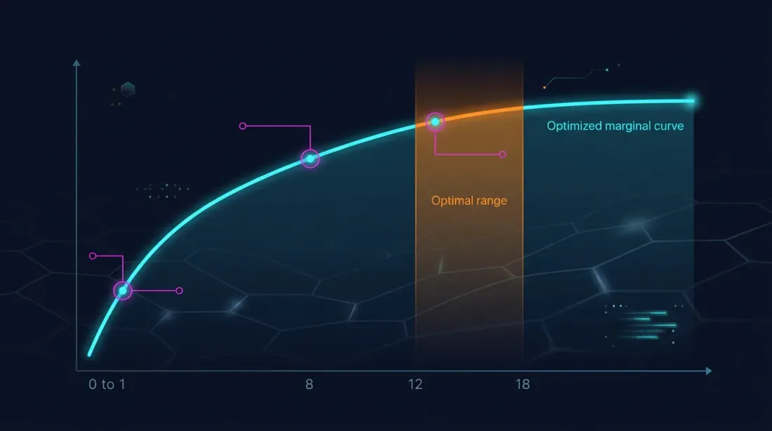
重要な問題:どのでもう1ペア追加してもfill_efficiencyが顕著に増加しなくなるのか?
import numpy as np

def diminishing_returns_analysis(
    trading_time_pct: float,
    correlation_factor: float = 3.0,
    max_pairs: int = 100,
    target_utilization: float = 0.80,
) -> dict:
    """
    Diminishing returns analysis from adding new pairs.
    """
    results = []
    target_n = None

    for n in range(1, max_pairs + 1):
        n_eff = n / correlation_factor
        p_active = 1 - (1 - trading_time_pct) ** n_eff
        marginal = 0
        if n > 1:
            prev_eff = (n - 1) / correlation_factor
            prev_p = 1 - (1 - trading_time_pct) ** prev_eff
            marginal = p_active - prev_p

        results.append({
            "n_pairs": n,
            "n_effective": n_eff,
            "p_at_least_one": p_active,
            "marginal_gain": marginal,
        })

        if target_n is None and p_active >= target_utilization:
            target_n = n

    return {
        "results": results,
        "target_n_for_utilization": target_n,
    }


analysis_b = diminishing_returns_analysis(0.05, correlation_factor=3.0, target_utilization=0.80)
print(f"Strategy B: need {analysis_b['target_n_for_utilization']} pairs for 80% P(≥1)")

for r in analysis_b["results"]:
    if r["n_pairs"] in [1, 3, 5, 10, 20, 30, 50, 80]:
        print(f"  N={r['n_pairs']:3d}: N_eff={r['n_effective']:.1f}, "
              f"P(≥1)={r['p_at_least_one']:.1%}, "
              f"marginal={r['marginal_gain']:.2%}")
戦略B(、)の結果:
| ペア | 限界利得 | ||
|---|---|---|---|
| 1 | 0.3 | 1.7% | — |
| 3 | 1.0 | 5.0% | +1.7% |
| 5 | 1.7 | 8.2% | +1.6% |
| 10 | 3.3 | 15.6% | +1.4% |
| 20 | 6.7 | 29.1% | +1.1% |
| 30 | 10.0 | 40.1% | +0.9% |
| 50 | 16.7 | 58.0% | +0.6% |
| 80 | 26.7 | 74.5% | +0.4% |
戦略Bの場合、80%のシングルスロット稼働率に到達することは100ペアでも不可能です(~96ペアが必要)。これは根本的な制約です:取引時間5%の戦略はシングルスロット運用には適していません — 複数の戦略を組み合わせたポートフォリオアプローチが必要です。
戦略A(、)の場合:
| ペア | 限界利得 | ||
|---|---|---|---|
| 5 | 1.7 | 23.6% | — |
| 10 | 3.3 | 41.8% | +3.3% |
| 20 | 6.7 | 65.9% | +2.1% |
| 30 | 10.0 | 80.3% | +1.2% |
戦略Aは~30ペアで80%の稼働率に到達します。30番目のペアの限界利得はわずか+1.2%です。
戦略C(、)の場合:
| ペア | ||
|---|---|---|
| 3 | 1.0 | 45.0% |
| 5 | 1.7 | 67.1% |
| 10 | 3.3 | 89.0% |
| 15 | 5.0 | 95.0% |
取引時間45%の戦略Cは、わずか10ペアで90%の稼働率に到達します。それ以上追加しても意味がありません。
ペア間のエッジ劣化

ペア数を制限するもう一つの要因があります:エッジの劣化。BTC/USDTで開発・最適化された戦略は、流動性の低いアルトコインではパフォーマンスが低下する可能性があります。
劣化の原因:
- 流動性:DOGE/USDTのスリッページはBTC/USDTの数倍
- スプレッド:流動性の低いペアはビッド・アスクスプレッドが広い
- マイクロストラクチャー:オーダーブックのパターンはペアによって異なる
- マニピュレーション:低流動性のアルトコインはポンプ・アンド・ダンプの影響を受けやすい
def edge_decay_analysis(
    strategy_results: dict,  # {pair: {"pnl_per_day": float, "n_trades": int}}
    min_trades: int = 30,
) -> list:
    """
    Rank pairs by edge accounting for degradation.
    """
    ranked = []
    for pair, metrics in strategy_results.items():
        if metrics["n_trades"] < min_trades:
            continue
        ranked.append({
            "pair": pair,
            "pnl_per_day": metrics["pnl_per_day"],
            "n_trades": metrics["n_trades"],
            "sharpe": metrics.get("sharpe", 0),
        })

    ranked.sort(key=lambda x: x["pnl_per_day"], reverse=True)

    cumulative_pnl = []
    running_sum = 0
    for i, r in enumerate(ranked):
        running_sum += r["pnl_per_day"]
        avg = running_sum / (i + 1)
        cumulative_pnl.append({
            "n_pairs": i + 1,
            "last_added": r["pair"],
            "last_pnl_per_day": r["pnl_per_day"],
            "avg_pnl_per_day": avg,
        })

    return cumulative_pnl
典型的な様相:
| ペア数 | 最後に追加 | 最後のPnL/日 | 平均PnL/日 |
|---|---|---|---|
| 1 | BTC/USDT | 0.89% | 0.89% |
| 2 | ETH/USDT | 0.82% | 0.86% |
| 3 | SOL/USDT | 0.71% | 0.81% |
| 5 | AVAX/USDT | 0.55% | 0.73% |
| 8 | DOT/USDT | 0.31% | 0.61% |
| 10 | DOGE/USDT | 0.12% | 0.53% |
10番目のペアを追加すると、ポートフォリオの平均PnL/日が下がります。8番目のペアの時点で、エッジはすでにベストの半分です。fill_efficiency(ペア数とともに増加)と平均エッジ(低下する)のバランスが必要です。
最適ペア数:統一モデル

fill_efficiencyとエッジ劣化を単一の指標 — 期待ポートフォリオPnL/日 — に統合します:
def optimal_pairs_count(
    pair_edges: list,           # PnL/day in descending order: [0.89, 0.82, 0.71, ...]
    trading_time_pct: float,
    correlation_factor: float = 3.0,
    max_slots: int = 1,
) -> dict:
    """
    Find the optimal number of pairs that maximizes portfolio PnL.
    """
    best_n = 0
    best_score = 0
    results = []

    for n in range(1, len(pair_edges) + 1):
        avg_edge = np.mean(pair_edges[:n])

        n_eff = n / correlation_factor
        p_active = 1 - (1 - trading_time_pct) ** n_eff
        expected_active = n_eff * trading_time_pct
        utilization = min(expected_active, max_slots) / max_slots
        fill_eff = min(p_active, utilization)

        portfolio_score = avg_edge * fill_eff * 365

        results.append({
            "n_pairs": n,
            "avg_edge": avg_edge,
            "fill_efficiency": fill_eff,
            "portfolio_annualized": portfolio_score,
        })

        if portfolio_score > best_score:
            best_score = portfolio_score
            best_n = n

    return {
        "optimal_n": best_n,
        "optimal_score": best_score,
        "results": results,
    }


edges = [0.89, 0.82, 0.71, 0.65, 0.55, 0.48, 0.40, 0.31, 0.22, 0.12,
         0.08, 0.05, 0.02, -0.01, -0.05]

opt = optimal_pairs_count(edges, trading_time_pct=0.15, correlation_factor=3.0)
print(f"Optimal number of pairs: {opt['optimal_n']}")
print(f"Portfolio annualized: {opt['optimal_score']:.1f}%")

for r in opt["results"]:
    print(f"  N={r['n_pairs']:2d}: avg_edge={r['avg_edge']:.2f}%, "
          f"fill_eff={r['fill_efficiency']:.1%}, "
          f"portfolio={r['portfolio_annualized']:.1f}%")
最適値は通常、ペア追加による限界fill_efficiencyが平均エッジの低下を補えなくなるポイントにあります。典型的な暗号通貨ポートフォリオの場合:
- 戦略B(5%時間):最適は8-12ペア
- 戦略A(15%時間):最適は6-10ペア
- 戦略C(45%時間):最適は4-6ペア
パラドックス:取引時間が最も短い戦略が最も多くのペアから恩恵を受けますが、fill_efficiencyは依然として低いままです。解決策はペアを増やすことではなく、他の戦略との組み合わせです(コンボ戦略を参照)。
クロスペア分散:相関削減戦略

ペア数を無限に増やせないなら、を下げる — つまりシグナルの多様性を高めることができます。
戦略1:流動性の高いトークンとDeFiトークンのミックス
BTC、ETH、BNBは非常に強く相関しています。しかし、UNI(DEX)、AAVE(レンディング)、CRV(ステーブルコイン)は独自のドライバーを持つ可能性があります。DeFiトークンを追加すると、平均が0.35から0.20-0.25に低下します:
戦略2:同じペアに異なる戦略
1つの戦略で10ペアではなく — 2つの異なる戦略で5ペア。戦略が異なる原理に基づいている場合(モメンタム vs. 平均回帰)、シグナルは逆相関になり得ます:
- モメンタムは価格上昇時にロングエントリー
- 平均回帰は価格下落時にロングエントリー
これはを達成する唯一の方法です — 負のシグナル相関を持つ戦略を使用することです。
戦略3:現物 vs. 先物
ファンディングレート裁定取引と現物取引は異なる相関構造を持っています。裁定戦略をポートフォリオに追加すると、全体のが大幅に低下します。裁定取引は定義上、収束ではなく乖離を利用するためです。
戦略タイプ別の実践的推奨事項
高頻度・低時間戦略(取引時間 < 10%)
典型的な代表:戦略B(5%時間、750日間で38トレード)。
- ペア数:10-15(エッジ/稼働バランスの最適値)
- 問題:15ペアでもfill_efficiencyは低い(~20-25%)
- 解決策:オーケストレーターで他の戦略との組み合わせが必須
- 暗号通貨の:2.5-3.5
- モニタリング:ローリングで市場レジームに応じたペア数の適応
中時間戦略(取引時間10-30%)
典型的な代表:戦略A(15%時間、750日間で418トレード)。
- ペア数:6-10
- 10ペアでのFill_efficiency:~40%
- 解決策:このような戦略を2-3組み合わせると80%以上の時間を埋められる
- 暗号通貨の:2.5-3.5
- 重点:最大エッジのペアを選択し、数を追わない
高時間戦略(取引時間 > 30%)
典型的な代表:戦略C(45%時間)。
- ペア数:4-6
- 6ペアでのFill_efficiency:~80%
- 問題:オーバーフロー — 複数ペアが同時にアクティブだがスロットが足りない
- 解決策:max_slotsを増やすかペア優先順位付けを追加
- 暗号通貨の:2.5-4.0(ロングポジションが危機と重なるため高い)
サマリーテーブル
| パラメータ | 戦略B(5%) | 戦略A(15%) | 戦略C(45%) |
|---|---|---|---|
| 推奨 | 10-15 | 6-10 | 4-6 |
| での | 3.3-5.0 | 2.0-3.3 | 1.3-2.0 |
| Fill eff.(1スロット) | 15-23% | 32-42% | 77-89% |
| 組み合わせ必要? | 必須 | 望ましい | 不要 |
| ボトルネック | シグナル不足 | バランス | オーバーフロー |
シリーズの他の指標との関連
この記事は「幻想なきバックテスト」シリーズの第11回です。シグナル相関は、前回の記事の指標に直接影響します:
-
PnL per Active Time: fill_efficiencyは実効リターン公式の主要な乗数です。相関を無視してfill_efficiencyを過大評価すると、ポートフォリオのPnL予測が過度に楽観的になります。
-
ファンディングレート: 高相関ではポジションが同時にオープンし、ファンディングコストはスロット数に比例して増大します。オーバーフロー + ファンディング = 資本の加速的な消耗。
-
ファンディングレート裁定: 裁定戦略はポートフォリオのを低下させる自然な分散要素です。そのシグナルはモメンタムや平均回帰戦略との相関が弱いです。
-
コンボ戦略(次の記事):異なるとを持つ戦略のポートフォリオを組み立てて90%以上の稼働率を達成する方法。カスケードオーケストレーションは優先度を割り当てる際にシグナル相関を考慮します。
結論
暗号通貨における分散はペア数の問題ではありません。10の相関ペアは3-4の独立したペアの効果しかもたらしません。パニック時にはさらに少なくなります。
4つの要点:
-
Nではなくeffective_Nを計算せよ。 暗号通貨ペアの。10ペアは~3.3の実効ペアです。fill_efficiencyはではなくに基づいて計画してください。
-
価格相関ではなくシグナル相関を測定せよ。 価格相関はプロキシであり、代替ではありません。すべてのペアで戦略を実行し、バイナリシグナル相関行列を計算してください。
-
エッジの劣化を考慮せよ。 ペアが増えると平均PnL/日が下がります。最適点は、新しいペアからの限界fill_efficiencyがエッジの低下を補えるポイントです。
-
を増やすのではなくを下げよ。 同じペアに異なる戦略を組み合わせる方が、1つの戦略をより多くのペアに適用するより効果的です。クロス戦略の分散はを達成できます。
Correlation factorは、稼働率とリターン予測がどれほど現実的かを決定する隠れた変数です。これを無視することは、幻想の上にポートフォリオを構築することを意味します。
参考リンク
- Markowitz, H. — Portfolio Selection (1952)
- López de Prado — Advances in Financial Machine Learning: Denoising and Detoning
- Ledoit, O. & Wolf, M. — Honey, I Shrunk the Sample Covariance Matrix (2004)
- Laloux, L. et al. — Noise Dressing of Financial Correlation Matrices (1999)
- Cont, R. — Empirical Properties of Asset Returns: Stylized Facts and Statistical Issues
- Ernest Chan — Algorithmic Trading: Portfolio Construction and Risk Management
- Rebonato, R. & Jäckel, P. — The Most General Methodology for Creating a Valid Correlation Matrix
Citation
@article{soloviov2026signalcorrelation,
  author = {Soloviov, Eugen},
  title = {Signal Correlation: How Many Pairs to Monitor},
  year = {2026},
  url = {https://marketmaker.cc/ru/blog/post/signal-correlation-pairs},
  version = {0.1.0},
  description = {Why 10 crypto pairs don't provide 10x diversification, how to calculate effective\_N via correlation\_factor, and how many pairs you really need to monitor for 80-90\% orchestrator slot utilization.}
}
MarketMaker.cc Team
クオンツ・リサーチ&戦略