Coordinate Descent vs Bayesian Optimization: Which Finds Better Parameters

This is the fifth article in the "Backtests Without Illusions" series. In previous articles we covered loss-profit asymmetry, Monte Carlo bootstrap, impact of funding rates, and Parquet cache for faster backtests. Now let's talk about the process of finding optimal strategy parameters — a task where intuition fails most often.
You have a strategy with 12 parameters. Each parameter takes ~9 values. You want to find the combination that maximizes PnL with limited drawdown. How do you do it?
If your answer is "I iterate through all combinations" — you have a problem. If your answer is "I change one parameter at a time" — you have a different problem. This article is about what problems lurk behind each approach and how to solve them.
Why Exhaustive Search Is Impossible

The Curse of Dimensionality
Exhaustive search (grid search) tests every combination of values for every parameter. For two parameters with 9 values, that's runs — perfectly feasible. For three: — tolerable.
But for a real strategy with 12 parameters:
Two hundred eighty-two billion runs. Even if a single backtest takes 1 second (which is already optimistic), exhaustive search would take:
This is exponential growth: each new parameter multiplies the search space by 9. Add a 13th parameter — and instead of 9,000 years you need 80,000.
import math

def grid_search_cost(n_params: int, values_per_param: int, seconds_per_trial: float) -> dict:
    """Estimate the cost of exhaustive search."""
    total_trials = values_per_param ** n_params
    total_seconds = total_trials * seconds_per_trial
    return {
        "total_trials": total_trials,
        "total_hours": total_seconds / 3600,
        "total_years": total_seconds / (3600 * 24 * 365),
    }

cost = grid_search_cost(12, 9, 1.0)
print(f"Trials: {cost['total_trials']:,.0f}")      # 282,429,536,481
print(f"Years:  {cost['total_years']:,.0f}")        # 8,950
Even with Precomputation
In the article about Parquet cache we showed how precomputing timeframes and indicators speeds up a single backtest to ~1 second. But even at 0.1 seconds per run, exhaustive search of 12 parameters would require 895 years. Precomputation helps, but doesn't solve the fundamental problem of exponential growth.
We need methods that explore the parameter space smarter than exhaustive search.
Coordinate Descent and OAT: Fast but Blind
Two Variants of the Same Idea
There are two related approaches — both optimize one parameter at a time, but differ in the number of passes:
OAT (One-at-a-Time) sweep — a single pass through all parameters. Iterate through values of the first parameter, fix the best, move to the second — and so on. Once. Fast and cheap.
Coordinate Descent — multi-pass. After optimizing the last parameter, return to the first and check whether the optimum has changed (since the context changed — other parameter values are now different). Repeat rounds until convergence. More expensive, but more precise — each round can refine the solution.
In practice, for backtests OAT is used more often: a single pass through 12 parameters — 96 runs. Coordinate descent with 3-5 rounds — 300-500 runs, which is already comparable to Optuna, but without its advantages.
For 12 parameters with ~8 values each:
Compare with for grid search. OAT is linear: instead of . This is both its main advantage and its main problem.
def oat_sweep(
    param_grid: dict[str, list],
    run_backtest_fn,
    initial_params: dict,
    metric: str = "effective_score",
) -> dict:
    """
    OAT sweep: single pass, optimizing one parameter at a time.

    param_grid: {"htf_entry_sell": [0.0, 0.005, ..., 0.05], ...}
    initial_params: starting values for all parameters
    metric: metric to optimize (effective_score recommended —
            PnL per active time extrapolated to a year)
    """
    best_params = initial_params.copy()
    best_score = run_backtest_fn(**best_params)[metric]

    for param_name, values in param_grid.items():
        param_best_val = best_params[param_name]
        param_best_score = best_score

        for val in values:
            candidate = best_params.copy()
            candidate[param_name] = val
            result = run_backtest_fn(**candidate)
            score = result[metric]

            if score > param_best_score:
                param_best_score = score
                param_best_val = val

        best_params[param_name] = param_best_val
        best_score = param_best_score
        print(f"{param_name}: best={param_best_val}, score={param_best_score:.4f}")

    return best_params
Which metric to choose for optimization? Instead of raw PnL or PnL@MaxLev, it is recommended to use effective score — PnL per active time extrapolated to a year. This metric accounts for time in position and allows correct comparison of strategies with different trading frequencies.
The Blind Spot: Parameter Interactions
OAT assumes that the effect of each parameter is additive — i.e., the optimal value of one parameter does not depend on the values of others. This assumption holds for some parameters, but breaks for coupled ones.
Additive vs Coupled Parameters
Before optimizing — it's useful to classify parameters:
Additive (independent) — the optimal value of one does not depend on the other. They can be optimized one at a time cheaply:
htf_entry_sellandhtf_entry_buy— entry thresholds for different directions (sell/buy) on the same timeframe. The sell threshold filters short signals, the buy threshold — longs. They operate on non-overlapping subsets of trades.tp_targetandbe_trigger— take-profit and breakeven, if they don't create conflicting exit conditions.
Coupled (interactive) — the optimal value of one depends on the other. Joint optimization is needed:
htf_entry_sellandmtf_entry_sell— thresholds for the same direction (sell) on different timeframes. HTF determines which signals reach MTF, and the MTF threshold determines filtering effectiveness. The HTF optimum shifts when MTF changes.ltf_entry_sell,mtf_entry_sell,htf_entry_sell— the entire threshold chain for one direction.partial_fracandtp_target— partial close size depends on the TP level.
Practical approach: first cheaply optimize additive parameters via OAT. Then optimize coupled groups via Optuna. This reduces the budget: instead of 12 parameters in Optuna, we send only 6-8 coupled ones, while the rest are already fixed.
Example: How OAT Misses an Interaction
Consider two coupled thresholds:
htf_entry_sell— threshold on the higher timeframe (sell direction)mtf_entry_sell— threshold on the middle timeframe (sell direction)
OAT fixes mtf_entry_sell = 0.01 (initial value) and iterates through htf_entry_sell. Finds the best value: htf_entry_sell = 0.02. Fixes it and moves to the next parameter — never returns.
Here's what OAT missed:
htf_entry_sell |
mtf_entry_sell |
PnL |
|---|---|---|
| 0.02 | 0.01 | +42% |
| 0.02 | 0.02 | +38% |
| 0.03 | 0.02 | +51% |
| 0.03 | 0.01 | +35% |
The combination (0.03, 0.02) yields PnL +51%, but OAT will never consider it because with fixed mtf_entry_sell = 0.01, the value htf_entry_sell = 0.03 yields only +35%. OAT got "stuck" in the local optimum (0.02, 0.01) and cannot see the global optimum (0.03, 0.02).
This is a classic problem: if the objective function landscape contains diagonal ridges (when the optimum of one parameter shifts as another changes), OAT misses them.
Formalizing the Problem
Let be the objective function (PnL). OAT finds a point where:
But this is a necessary, not sufficient condition for a global optimum. If the Hessian matrix has significant off-diagonal elements — OAT does not account for cross-derivatives when .
For coupled parameters (thresholds of the same direction across multiple timeframes) — interactions are the rule, not the exception. The entry threshold on the higher timeframe determines which signals reach the middle one, and the threshold on the middle one determines filtering effectiveness on the lower. For additive parameters (different directions, independent filters) cross-derivatives are close to zero — and OAT works well.
Bayesian Optimization: Smart Search

The Idea
Instead of blind enumeration or greedy search, Bayesian optimization builds a surrogate model of the objective function and at each step selects the point where the expected improvement is maximum.
Algorithm:
- Choose several random points, evaluate the objective function
- Build a surrogate model (approximates from observed points)
- Find the point with maximum expected improvement (acquisition function)
- Evaluate the objective function at that point
- Update the surrogate model
- Repeat steps 3-5
The key difference from OAT: Bayesian optimization considers all parameters simultaneously and can explore diagonal ridges in parameter space.
TPE (Tree-structured Parzen Estimator)

TPE is the default sampler in Optuna. Instead of modeling directly, TPE models two distributions:
- — distribution of parameters where the objective function is better than threshold
- — distribution of parameters where the objective function is worse than threshold
TPE's acquisition function — the ratio:
TPE selects points where is large (parameters similar to "good" ones) and is small (parameters not similar to "bad" ones).
Why TPE is suitable for backtests:
- Handles conditional dependencies between parameters
- Does not require continuity of the objective function
- Efficient with moderate budgets (100-1000 iterations)
- Supports categorical and discrete parameters
Gaussian Process (GP)
An alternative to TPE — Gaussian Process. GP models as a multivariate normal process and provides not only a value prediction, but also uncertainty at each point.
where is the mean, is the covariance function (kernel).
GP works well when:
- There are few parameters (up to 10-15)
- The objective function is smooth
- Each run is expensive (minutes, hours)
For backtests with a precomputed Parquet cache, where a single run takes ~1 second, TPE is usually preferred: it builds the model faster and scales better to 500+ iterations.
Practical Integration with Optuna

Full Working Example
import optuna
from optuna.samplers import TPESampler
import numpy as np


def run_backtest(htf_pre, mtf_pre, ltf_pre, **params) -> dict:
    """
    Runs a backtest with given parameters.
    Returns a dict with metrics: pnl, max_dd, n_trades, trading_time, sharpe.
    Uses precomputed Parquet cache — ~1 second per run.
    """
    pass


def objective(trial: optuna.Trial) -> float:
    """Objective function for Optuna."""
    params = {
        "htf_entry_sell": trial.suggest_float("htf_entry_sell", 0.0, 0.05, step=0.005),
        "htf_entry_buy":  trial.suggest_float("htf_entry_buy",  0.0, 0.05, step=0.005),

        "mtf_entry_sell": trial.suggest_float("mtf_entry_sell", 0.0, 0.05, step=0.005),
        "mtf_entry_buy":  trial.suggest_float("mtf_entry_buy",  0.0, 0.05, step=0.005),

        "ltf_entry_sell": trial.suggest_float("ltf_entry_sell", 0.0, 0.05, step=0.005),
        "ltf_entry_buy":  trial.suggest_float("ltf_entry_buy",  0.0, 0.05, step=0.005),

        "htf_exit_sell":  trial.suggest_float("htf_exit_sell",  0.0, 0.03, step=0.005),
        "htf_exit_buy":   trial.suggest_float("htf_exit_buy",   0.0, 0.03, step=0.005),
        "mtf_exit_sell":  trial.suggest_float("mtf_exit_sell",  0.0, 0.03, step=0.005),
        "mtf_exit_buy":   trial.suggest_float("mtf_exit_buy",   0.0, 0.03, step=0.005),

        "min_hold_bars":  trial.suggest_int("min_hold_bars", 1, 20),
        "trail_pct":      trial.suggest_float("trail_pct", 0.001, 0.02, step=0.001),
    }

    result = run_backtest(htf_pre, mtf_pre, ltf_pre, **params)

    return -result["pnl_at_max_lev"]


study = optuna.create_study(
    sampler=TPESampler(seed=42),
    study_name="strategy_optimization",
    direction="minimize",
)

study.optimize(objective, n_trials=500, show_progress_bar=True)

print(f"Best PnL: {-study.best_value:.2f}%")
print(f"Best params: {study.best_params}")
print(f"Total trials: {len(study.trials)}")
At ~1 second per backtest (with precomputed cache):
Eight minutes versus 8,950 years of exhaustive search. And TPE in 500 iterations finds combinations that OAT misses in 96, because it explores the parameter space simultaneously rather than one axis at a time.
Saving and Resuming a Study
import optuna

study = optuna.create_study(
    storage="sqlite:///optuna_study.db",
    study_name="strategy_v2",
    sampler=TPESampler(seed=42),
    direction="minimize",
    load_if_exists=True,  # continue if study already exists
)

study.optimize(objective, n_trials=300)


study.optimize(objective, n_trials=200)
Adding Constraints
Not all parameter combinations are valid. For example, the exit threshold should not exceed the entry threshold:
def objective_with_constraints(trial: optuna.Trial) -> float:
    htf_entry = trial.suggest_float("htf_entry_sell", 0.0, 0.05, step=0.005)
    htf_exit  = trial.suggest_float("htf_exit_sell",  0.0, 0.03, step=0.005)

    if htf_exit > htf_entry:
        raise optuna.TrialPruned()

    result = run_backtest(htf_pre, mtf_pre, ltf_pre, **params)
    return -result["pnl_at_max_lev"]
Sampler Comparison

Optuna supports several samplers. Each has its own strengths.
TPESampler (default)
sampler = optuna.samplers.TPESampler(
    n_startup_trials=20,  # random trials before modeling begins
    seed=42,
)
- Principle: Tree-structured Parzen Estimator
- Strengths: good for mixed parameter types, scales to 1000+ iterations
- Weaknesses: may be less efficient with strong parameter interactions
- When to use: by default, if there's no reason to choose another
CmaEsSampler
sampler = optuna.samplers.CmaEsSampler(seed=42)
- Principle: Covariance Matrix Adaptation Evolution Strategy — an evolutionary algorithm that adapts the covariance matrix
- Strengths: excellent at finding interactions between continuous parameters, accounts for correlations
- Weaknesses: does not support categorical parameters, requires more iterations for initialization
- When to use: if all parameters are continuous and you suspect strong interactions
GPSampler
sampler = optuna.samplers.GPSampler(seed=42)
- Principle: Gaussian Process with acquisition function
- Strengths: best sample efficiency (fewer iterations for a good result), provides uncertainty estimates
- Weaknesses: in iteration count — slow when
- When to use: if a single backtest is expensive (minutes) and the budget is limited to 100-200 iterations
RandomSampler (baseline)
sampler = optuna.samplers.RandomSampler(seed=42)
- Principle: uniform random sampling
- Strengths: doesn't get stuck in local optima, full space coverage
- Weaknesses: doesn't use previous results
- When to use: as a baseline for comparison, or for exploratory analysis
QMCSampler
sampler = optuna.samplers.QMCSampler(seed=42)
- Principle: Quasi-Monte Carlo (Sobol/Halton sequences) — fills the space more uniformly than a random sampler
- Strengths: better space coverage than RandomSampler, reproducibility
- Weaknesses: does not adapt to results
- When to use: for the first 50-100 iterations before switching to TPE
Summary Table
| Sampler | Type | Interactions | Categorical | Best Budget |
|---|---|---|---|---|
| TPE | Bayesian | Partial | Yes | 100-1000 |
| CmaEs | Evolutionary | Yes | No | 200-2000 |
| GP | Bayesian | Yes | Limited | 50-200 |
| Random | Random | No | Yes | Any (baseline) |
| QMC | Quasi-random | No | No | 50-500 |
Practical Benchmark
import optuna
import time

def benchmark_sampler(sampler, n_trials=300):
    """Compare samplers on the same task."""
    study = optuna.create_study(sampler=sampler, direction="minimize")

    start = time.time()
    study.optimize(objective, n_trials=n_trials, show_progress_bar=False)
    elapsed = time.time() - start

    return {
        "best_value": -study.best_value,
        "elapsed_sec": elapsed,
        "best_trial": study.best_trial.number,
    }

samplers = {
    "TPE":    optuna.samplers.TPESampler(seed=42),
    "CmaEs":  optuna.samplers.CmaEsSampler(seed=42),
    "GP":     optuna.samplers.GPSampler(seed=42),
    "Random": optuna.samplers.RandomSampler(seed=42),
    "QMC":    optuna.samplers.QMCSampler(seed=42),
}

for name, sampler in samplers.items():
    result = benchmark_sampler(sampler, n_trials=300)
    print(f"{name:8s}: best PnL={result['best_value']:.2f}%, "
          f"found at trial #{result['best_trial']}, "
          f"time={result['elapsed_sec']:.1f}s")
Typical results for a strategy with 12 parameters:
| Sampler | Best PnL | Found at Iteration | Sampler Overhead |
|---|---|---|---|
| TPE | ~51% | ~180 | Low |
| CmaEs | ~49% | ~250 | Medium |
| GP | ~48% | ~90 | High when |
| Random | ~42% | ~270 | Minimal |
| QMC | ~43% | ~200 | Minimal |
TPE and CmaEs consistently outperform random search by 15-20% in final PnL. GP finds good results earlier but hits a computational ceiling with a large number of iterations.
Multi-Objective Optimization: PnL vs MaxDD
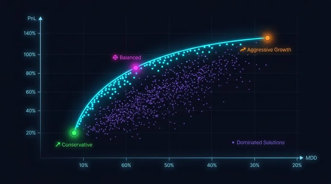
Why a Single Criterion Is Not Enough
Maximizing PnL without drawdown constraints is a path to disaster. A strategy with PnL +80% and MaxDD -30% is, due to loss-profit asymmetry, significantly riskier than a strategy with PnL +50% and MaxDD -5%.
The optimization problem is actually multi-objective:
These goals conflict: aggressive parameters increase both PnL and drawdown. The solution is not a single point, but a Pareto front: a set of solutions where you cannot improve one metric without worsening the other.
NSGA-II / NSGA-III in Optuna
import optuna

def multi_objective(trial: optuna.Trial) -> tuple[float, float]:
    """Multi-objective function: (PnL, MaxDD)."""
    params = {
        "htf_entry_sell": trial.suggest_float("htf_entry_sell", 0.0, 0.05, step=0.005),
        "htf_entry_buy":  trial.suggest_float("htf_entry_buy",  0.0, 0.05, step=0.005),
        "mtf_entry_sell": trial.suggest_float("mtf_entry_sell", 0.0, 0.05, step=0.005),
        "mtf_entry_buy":  trial.suggest_float("mtf_entry_buy",  0.0, 0.05, step=0.005),
        "ltf_entry_sell": trial.suggest_float("ltf_entry_sell", 0.0, 0.05, step=0.005),
        "ltf_entry_buy":  trial.suggest_float("ltf_entry_buy",  0.0, 0.05, step=0.005),
        "htf_exit_sell":  trial.suggest_float("htf_exit_sell",  0.0, 0.03, step=0.005),
        "htf_exit_buy":   trial.suggest_float("htf_exit_buy",   0.0, 0.03, step=0.005),
        "mtf_exit_sell":  trial.suggest_float("mtf_exit_sell",  0.0, 0.03, step=0.005),
        "mtf_exit_buy":   trial.suggest_float("mtf_exit_buy",   0.0, 0.03, step=0.005),
        "min_hold_bars":  trial.suggest_int("min_hold_bars", 1, 20),
        "trail_pct":      trial.suggest_float("trail_pct", 0.001, 0.02, step=0.001),
    }

    result = run_backtest(htf_pre, mtf_pre, ltf_pre, **params)

    pnl = result["pnl"]          # maximize
    max_dd = result["max_dd"]    # minimize (already a negative number)

    return pnl, max_dd  # Optuna: both directions are set in create_study


study = optuna.create_study(
    directions=["maximize", "minimize"],
    sampler=optuna.samplers.NSGAIIISampler(seed=42),
    study_name="multi_objective_strategy",
)

study.optimize(multi_objective, n_trials=500)

pareto_trials = study.best_trials
print(f"Pareto front: {len(pareto_trials)} solutions")

for t in pareto_trials[:5]:
    print(f"  PnL={t.values[0]:.2f}%, MaxDD={t.values[1]:.2f}%")
Selecting a Point on the Pareto Front
The Pareto front gives multiple solutions. How to choose one?
def select_from_pareto(
    pareto_trials: list,
    max_dd_limit: float = -5.0,
    min_pnl: float = 20.0,
) -> list:
    """
    Filter the Pareto front by constraints.

    max_dd_limit: maximum acceptable drawdown (e.g., -5%)
    min_pnl: minimum acceptable PnL (%)
    """
    filtered = []
    for trial in pareto_trials:
        pnl, max_dd = trial.values
        if max_dd >= max_dd_limit and pnl >= min_pnl:
            max_lev = min(50 / abs(max_dd), 100) if max_dd != 0 else 100
            pnl_at_max_lev = pnl * max_lev
            filtered.append({
                "trial": trial,
                "pnl": pnl,
                "max_dd": max_dd,
                "max_lev": max_lev,
                "pnl_at_max_lev": pnl_at_max_lev,
            })

    filtered.sort(key=lambda x: x["pnl_at_max_lev"], reverse=True)
    return filtered
Note: when calculating PnL at maximum leverage, you must account for funding rates, otherwise theoretically high leverage will turn into a loss on the real market. Additionally, the final PnL is a single-point estimate, and to assess result stability you need Monte Carlo bootstrap.
Example: Three Strategies on the Pareto Front
| Strategy | PnL | MaxDD | MaxLev | PnL@MaxLev | Trading time |
|---|---|---|---|---|---|
| Strategy A | ~55% | ~0.9% | ~55x | ~3025% | ~15% |
| Strategy B | ~25% | ~0.75% | ~66x | ~1650% | ~5% |
| Strategy C | ~300% | ~17% | ~3x | ~900% | ~45% |
Strategy C with an impressive PnL of +300% turns out to be the least attractive by PnL@MaxLev due to high drawdown. Strategy A leads in net leveraged return, but when accounting for PnL per active time, Strategy B may be preferable — 95% of free time can be filled with other strategies.
Contour Plots and Parameter Importance

Landscape Visualization
After optimization — visualization. Optuna provides built-in tools:
import optuna.visualization as vis

fig_contour = vis.plot_contour(
    study,
    params=["htf_entry_sell", "mtf_entry_sell"],
)
fig_contour.show()

fig_importance = vis.plot_param_importances(study)
fig_importance.show()

fig_history = vis.plot_optimization_history(study)
fig_history.show()

fig_parallel = vis.plot_parallel_coordinate(
    study,
    params=["htf_entry_sell", "mtf_entry_sell", "ltf_entry_sell"],
)
fig_parallel.show()

fig_slice = vis.plot_slice(study)
fig_slice.show()
Contour Plot: Reading Interactions
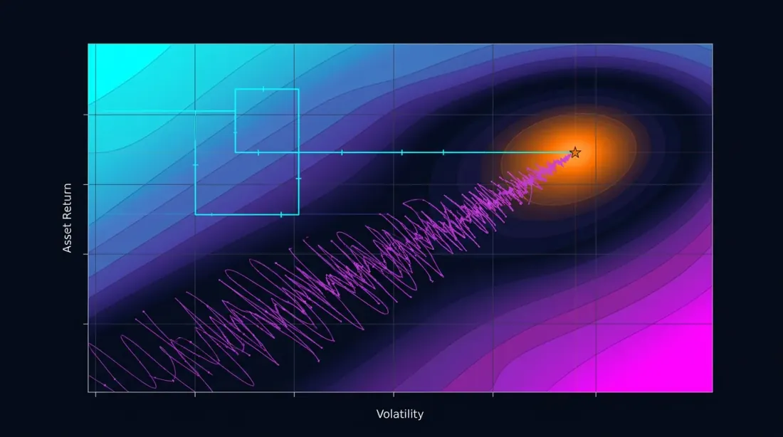
A contour plot builds a two-dimensional cross-section of the objective function for a pair of parameters. If the isolines are parallel to one of the axes — the parameters don't interact, and OAT would have found the same optimum. If the isolines are diagonal — there is interaction, and OAT will miss.
key_params = ["htf_entry_sell", "mtf_entry_sell", "ltf_entry_sell",
              "htf_entry_buy",  "mtf_entry_buy",  "ltf_entry_buy"]

for i, p1 in enumerate(key_params):
    for p2 in key_params[i+1:]:
        fig = vis.plot_contour(study, params=[p1, p2])
        fig.write_image(f"contour_{p1}_vs_{p2}.png")
If a contour plot shows a plateau — a region where the objective function changes little — this is a good sign. A plateau means the result is robust to small parameter deviations. More about plateau analysis and its relationship to overfitting — in the upcoming article Plateau analysis.
Parameter Importance
importance = optuna.importance.get_param_importances(study)
for param, imp in importance.items():
    print(f"{param:20s}: {imp:.4f}")
Typical output:
htf_entry_sell      : 0.2841
mtf_entry_sell      : 0.2103
ltf_entry_sell      : 0.1567
trail_pct           : 0.1204
htf_entry_buy       : 0.0892
...
Parameters with importance < 0.01 can be fixed at their default value — this reduces the dimensionality of the problem and speeds up optimization. But be careful: low importance may also mean the parameter is important only in interaction with others. Verify through contour plots.
Precomputed Cache: Why 1 Second per Backtest Changes Everything

The speed of a single backtest determines which optimization method you can afford.
| Backtest Time | 96 OAT | 500 TPE | 2000 CmaEs |
|---|---|---|---|
| 60 seconds | 1.6 hours | 8.3 hours | 33 hours |
| 10 seconds | 16 minutes | 83 minutes | 5.5 hours |
| 1 second | 1.5 minutes | 8 minutes | 33 minutes |
| 0.1 seconds | 10 seconds | 50 seconds | 3.3 minutes |
At 60 seconds per backtest, 500 TPE iterations take 8 hours. Already tolerable, but iterating (changing the objective function, restarting) is expensive. At 1 second — 8 minutes, and you can run dozens of experiments per day.
This is precisely why precomputation into Parquet cache is not just a speed optimization, but an expansion of the space of available methods. Without cache you're limited to OAT or 100 GP iterations. With cache — you can afford 2000 CmaEs iterations or a full multi-objective NSGA-III.
import pyarrow.parquet as pq
import time

t0 = time.time()
htf_pre = pq.read_table("cache/htf_indicators.parquet").to_pandas()
mtf_pre = pq.read_table("cache/mtf_indicators.parquet").to_pandas()
ltf_pre = pq.read_table("cache/ltf_indicators.parquet").to_pandas()
print(f"Cache loaded in {time.time() - t0:.2f}s")  # ~0.3s

t1 = time.time()
result = run_backtest(htf_pre, mtf_pre, ltf_pre, htf_entry_sell=0.02, ...)
print(f"Backtest in {time.time() - t1:.2f}s")  # ~1.0s
Practical Recommendations

When to Use OAT
OAT is justified in the following cases:
-
Exploratory analysis. You're just starting to explore a strategy and want to understand which parameters affect the result at all. 96 runs in 1.5 minutes — an excellent starting point.
-
Additive parameters. For parameters that operate on non-overlapping subsets of trades (sell vs buy directions, different instruments), OAT will give a correct result faster.
-
Very expensive backtest. If a single run takes 10+ minutes and cannot be sped up, OAT with 96 runs (16 hours) is preferable to 500 TPE iterations (3.5 days).
When to Use Optuna
Optuna is preferable in most cases:
-
More than 3 parameters. Interactions are practically guaranteed — OAT will miss the optimum.
-
Multi-timeframe strategies. Thresholds across different timeframes are almost always interconnected.
-
Final optimization. When the strategy has passed Monte Carlo bootstrap and you're confident in its robustness — Optuna will find the best parameters.
-
Multi-objective problems. PnL vs MaxDD vs trading time — OAT cannot solve this problem in principle.
Hybrid Approach: OAT for Additive + Optuna for Coupled
You don't have to choose between OAT and Optuna — it's better to combine them:
-
Classify parameters. Divide into additive (independent) and coupled (interactive). Example for 12 separation parameters:
- Additive:
htf_entry_sell<->htf_entry_buy,mtf_entry_sell<->mtf_entry_buy,ltf_entry_sell<->ltf_entry_buy(sell/buy — different directions, operate on non-overlapping trades) - Coupled group sell:
htf_entry_sell,mtf_entry_sell,ltf_entry_sell(filtering chain: HTF -> MTF -> LTF for sell signals) - Coupled group buy:
htf_entry_buy,mtf_entry_buy,ltf_entry_buy
- Additive:
-
OAT for additive. Optimize sell and buy groups independently. If sell parameters don't affect buy trades — OAT will give a correct result in minutes.
-
Optuna for coupled. Within each group (sell: 6 parameters entry+exit) use TPE. 6 parameters instead of 12 — the budget is cut in half.
sell_params = oat_sweep(sell_param_grid, run_backtest, initial_params)

def objective_sell(trial):
    params = sell_params.copy()
    params["htf_entry_sell"] = trial.suggest_float("htf_entry_sell", 0.0, 0.05, step=0.005)
    params["mtf_entry_sell"] = trial.suggest_float("mtf_entry_sell", 0.0, 0.05, step=0.005)
    params["ltf_entry_sell"] = trial.suggest_float("ltf_entry_sell", 0.0, 0.05, step=0.005)
    params["htf_exit_sell"] = trial.suggest_float("htf_exit_sell", 0.0, 0.02, step=0.001)
    params["mtf_exit_sell"] = trial.suggest_float("mtf_exit_sell", 0.0, 0.02, step=0.001)
    params["ltf_exit_sell"] = trial.suggest_float("ltf_exit_sell", 0.0, 0.02, step=0.001)
    return -run_backtest(**params)["effective_score"]

study = optuna.create_study(sampler=optuna.samplers.TPESampler())
study.optimize(objective_sell, n_trials=300)  # 6 parameters → 300 is enough
Full Optimization Pipeline
1. Precompute Parquet cache (once)
2. Classify parameters: additive vs coupled
3. OAT for additive (~50 runs, ~1 min) → fix
4. Optuna TPE for coupled groups (300 iterations x 2 groups, ~10 min)
5. Optuna NSGA-III for meta-parameters (500 iterations, ~8 min) → Pareto front
6. Contour plots → visualize interactions
7. Monte Carlo bootstrap of best points → confidence intervals
8. Walk-Forward → out-of-sample validation
Step 8 — walk-forward optimization — is critically important for protection against overfitting. More about this in the upcoming article Walk-Forward.
Optimization Pitfalls
Overfitting. The more parameters and the more precise the optimization — the higher the risk of fitting the strategy to historical data. 500 Optuna iterations with 12 parameters will find a combination that works perfectly on the training set, but is useless on new data.
Protection:
- Split data into train/test (70/30)
- Use Monte Carlo bootstrap to assess stability
- Validate through walk-forward
- Prefer solutions on plateaus (more about this in Plateau analysis)
Multiple comparisons problem. If you test 500 combinations, the probability of randomly finding a "good" result grows. Bonferroni correction or FDR (False Discovery Rate) control help, but the simpler approach is out-of-sample validation.
Insufficient budget. TPE with 50 iterations for 12 parameters is too few. The first 20 iterations are random (startup), leaving only 30 for modeling. Minimum budget: iterations for 12 parameters, recommended: .
Freqtrade: How It Works in a Production Framework

Freqtrade — one of the popular algotrading frameworks — uses Optuna under the hood through the Hyperopt module. Its experience confirms our recommendations:
- Samplers: TPE (default), GP, CmaEs, NSGA-II, QMC — all available through configuration
- Loss functions: 12 built-in loss functions, including ShortTradeDurHyperOptLoss, SharpeHyperOptLoss, MaxDrawDownHyperOptLoss
- Multi-objective: support for NSGA-II and NSGA-III for simultaneous optimization of multiple metrics
- Custom samplers: ability to plug in any Optuna-compatible sampler
A key lesson from the Freqtrade ecosystem: built-in loss functions cover typical scenarios, but for serious optimization you need a custom objective function that accounts for your strategy's specifics — active time, funding costs, adaptive drill-down for accurate fill simulation.
Conclusion

Coordinate descent (OAT) is a fast and intuitive method. For 12 parameters it requires only 96 runs and finishes in a minute and a half. But it is blind to parameter interactions — and in multi-timeframe strategies, interactions are almost always present.
Bayesian optimization through Optuna (TPE, GP, CmaEs) explores the parameter space as a whole. 500 iterations in 8 minutes — with a precomputed Parquet cache — find combinations invisible to OAT.
Multi-objective optimization (NSGA-III) transforms the problem of "maximize PnL" into the problem of "build a Pareto front of PnL vs MaxDD" — and provides a set of solutions with different risk-return tradeoffs.
But optimization is only part of the pipeline. The found parameters need to be validated through Monte Carlo bootstrap, corrected for funding rates, recalculated accounting for active time, and run through walk-forward validation. More on that in the upcoming articles of the series.
Useful Links
- Optuna: A Next-generation Hyperparameter Optimization Framework (Akiba et al., 2019)
- Algorithms for Hyper-Parameter Optimization (Bergstra et al., 2011) — the original TPE paper
- Optuna Documentation — Samplers
- Optuna Visualization Module
- Hansen, N. — The CMA Evolution Strategy: A Tutorial
- Deb, K. et al. — NSGA-II: A Fast and Elitist Multiobjective Genetic Algorithm (2002)
- Snoek, J. et al. — Practical Bayesian Optimization of Machine Learning Algorithms (2012)
- Freqtrade Documentation — Hyperopt
- Marcos Lopez de Prado — Advances in Financial Machine Learning, Chapter 12
- Bergstra, J. & Bengio, Y. — Random Search for Hyper-Parameter Optimization (2012)
Citation
@article{soloviov2026optuna,
  author = {Soloviov, Eugen},
  title = {Coordinate Descent vs Bayesian Optimization: Which Finds Better Parameters},
  year = {2026},
  url = {https://marketmaker.cc/en/blog/post/optuna-vs-coordinate-descent},
  description = {Why exhaustive search is impossible for 12+ parameters, how coordinate descent misses interactions, and how Optuna with a TPE sampler finds in 500 iterations what OAT cannot find in 96.}
}
MarketMaker.cc Team
Сандық зерттеулер және стратегия
Read More

Adaptive Drill-Down: Backtest with Variable Granularity from Minutes to Raw Trades

Aggregated Parquet Cache: How to Speed Up Multi-Timeframe Backtests by Hundreds of Times