Koopman Operators and DMD: Do Market Modes Survive Out-of-Sample?

Dynamic Mode Decomposition आपको एक spectrum देता है: कुछ complex eigenvalues, जिनमें प्रत्येक की growth rate और frequency होती है, और प्रत्येक आपके asset cross-section पर एक spatial mode से जुड़ा होता है। यह किसी structure जैसा दिखता है। पूरा सवाल यह है कि क्या यह वास्तव में structure है, या कोई linear operator noise की एक window को कर्तव्यपूर्वक याद कर रहा है।
इस सवाल के दो testable हिस्से हैं, और यह लेख इन्हीं के आसपास बनाया गया है:
- Mode persistence. Window और window पर DMD fit करें। क्या dominant modes एक ही subspace को span करते हैं, या हर refit पर बदल जाते हैं? यदि वे बदलते हैं, तो DMD in-sample decomposition है और कुछ अधिक नहीं — इसे साफ-साफ कहना एक और tutorial से अधिक उपयोगी है।
- Leading indicator के रूप में spectral radius. सबसे बड़ा eigenvalue modulus fitted dynamics की explosiveness को सारांशित करने वाला एक scalar है। क्या यह realised volatility को lead करता है, lag करता है, या केवल उसे दोहराता है? कोई भी उत्तर publishable है; केवल पहला tradeable है।
बाजार non-stationary nonlinear systems हैं, यह यहां मान लिया गया है, तर्क नहीं दिया गया — blog ने इसे पहले ही algotrading में attractors में phase-space geometry के साथ और HMMs के साथ regime detection में मापे गए per-regime BTC statistics के साथ समझाया है। आगे का प्रश्न संकरा है: non-stationarity fitted Koopman operator के साथ क्या करती है, और इसे कैसे मापा जाए।
1. मूल विचार: Nonlinear Dynamics को Linear बनाना
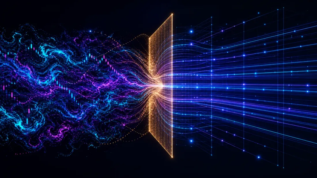
State space पर discrete-time dynamical system पर विचार करें:
जहां संभवतः nonlinear map है। बाजारों के लिए, समय step पर asset returns, volatilities या order-book imbalances का vector है।
Koopman operator सीधे state पर नहीं, बल्कि scalar-valued observable functions पर काम करता है:
मुख्य गुण: linear है, भले ही न हो। इसकी कीमत dimensionality है — infinite-dimensional function space पर काम करता है। एक अच्छा finite-dimensional approximation nonlinear dynamics की expressiveness को linear algebra की tractability के साथ जोड़ता है: prediction matrix exponentiation बन जाता है, और हर mode inspectable होता है, network weights में छिपा नहीं रहता।
2. Koopman Operator का Spectral Decomposition
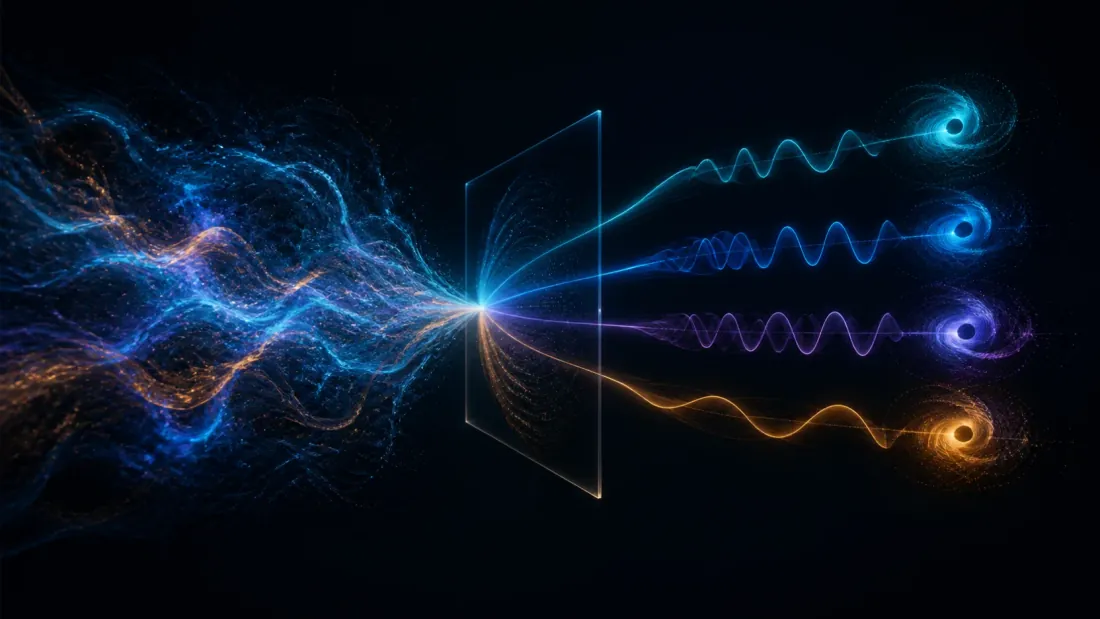
यदि के eigenvalues और eigenfunctions हैं, तो , और इन eigenfunctions के span में कोई भी observable इस प्रकार decompose होता है:
जहां Koopman modes हैं — vector-valued coefficients जो बताते हैं कि प्रत्येक eigenfunction पूरे observable vector में कैसे योगदान देती है।
प्रत्येक eigenvalue growth या decay rate () और oscillation frequency () encode करता है:
| Component | Eigenvalue property | Financial interpretation |
|---|---|---|
| Trend | , | Slow drift, momentum |
| Cycles | , | Oscillations, seasonality |
| Transients | Decaying shocks, short-lived moves | |
| Unstable modes | Growing, explosive dynamics |
यह table promise है। Section 4 में उस promise को data के विरुद्ध जांचा जाएगा।
3. Dynamic Mode Decomposition (DMD)
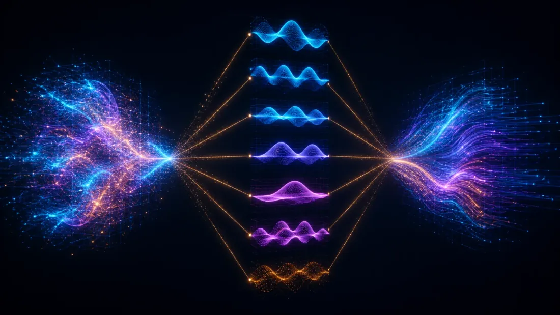
DMD data से का approximation निकालने का workhorse algorithm है। Matrices में व्यवस्थित snapshots दिए हों:
DMD best-fit linear operator को के साथ खोजता है:
- SVD निकालें:
- Project करें:
- Eigendecompose करें:
- Full-space modes वापस पाएं:
के columns DMD modes हैं; के diagonal में DMD eigenvalues होते हैं।
import numpy as np
from numpy.linalg import svd, eig, lstsq

def dmd(X: np.ndarray, rank: int | None = None) -> tuple:
    """
    Dynamic Mode Decomposition.

    Parameters
    ----------
    X : np.ndarray, shape (n_features, n_snapshots)
        Data matrix where each column is a state snapshot.
    rank : int or None
        Truncation rank for the SVD. None = no truncation.

    Returns
    -------
    eigenvalues : np.ndarray, shape (r,)
        DMD eigenvalues (approximating Koopman eigenvalues).
    modes : np.ndarray, shape (n_features, r)
        DMD modes (columns), L2-normalised.
    amplitudes : np.ndarray, shape (r,)
        Mode amplitudes fitted to the FINAL snapshot, so that a one-step
        forecast is simply modes @ (eigenvalues * amplitudes).
    """
    X0 = X[:, :-1]
    X1 = X[:, 1:]

    U, S, Vh = svd(X0, full_matrices=False)

    if rank is not None:
        U = U[:, :rank]
        S = S[:rank]
        Vh = Vh[:rank, :]

    S_inv = np.diag(1.0 / S)

    A_tilde = U.conj().T @ X1 @ Vh.conj().T @ S_inv
    eigenvalues, W = eig(A_tilde)

    modes = X1 @ Vh.conj().T @ S_inv @ W

    norms = np.linalg.norm(modes, axis=0)
    norms[norms == 0] = 1.0
    modes = modes / norms

    amplitudes = lstsq(modes, X[:, -1].astype(complex), rcond=None)[0]

    return eigenvalues, modes, amplitudes
यहां दो जानबूझकर किए गए चुनाव हैं। Modes को L2-normalised किया गया है, क्योंकि section 4.2 windows के बीच mode subspaces की तुलना करता है और unnormalised amplitudes तुलना पर हावी हो जाते। Amplitudes को first के बजाय last snapshot पर fit किया गया है, जिसका अर्थ है कि forecast कभी eigenvalue को बड़ी power तक नहीं उठाता — यही वह numerical blow-up का स्रोत है जो naive DMD signals को dynamics जैसा दिखाता है जबकि वे floating-point overflow होते हैं।
4. Measurement
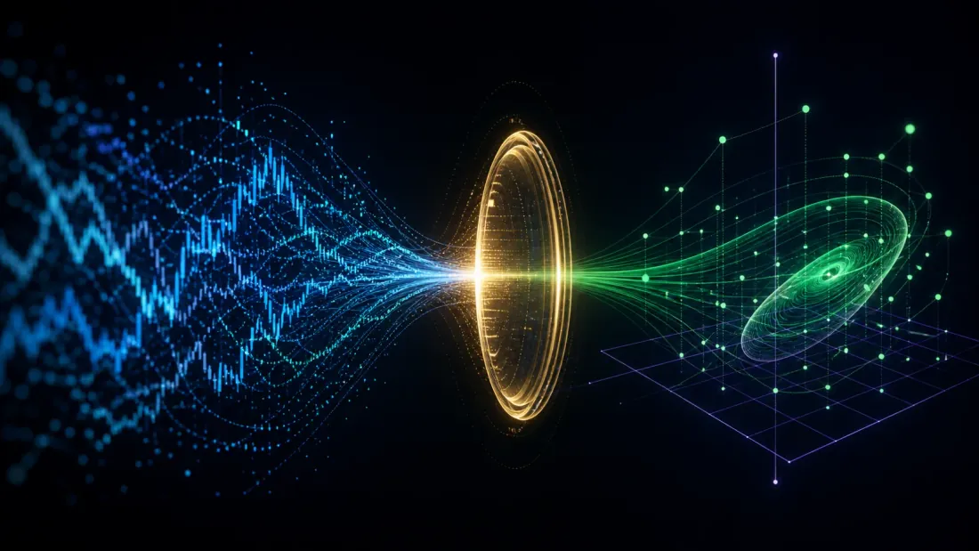
यह लेख का वह हिस्सा है जो textbook नहीं है। ऊपर सब कुछ fitting procedure है; नीचे यह पता लगाने का protocol है कि fit का कोई अर्थ है या नहीं।
Data. Project के अपने exchange data का उपयोग करें — consistent minute या tick grid पर BTC, ETH और liquid alts का cross-section, equity ETFs का daily download नहीं। Blog crypto-first है और microstructure का तर्क सीधे transfer नहीं होता। को rows पर assets और columns पर time के साथ log returns में बनाएं, हर window के भीतर per asset demeaned।
4.1 Eigenvalue spectrum
एक representative window के लिए report करें: eigenvalues में से कितने unit circle की tolerance के भीतर आते हैं, प्रत्येक hours में किस oscillation period से मेल खाता है (period bars, converted), और top modes return variance का कितना fraction reconstruct करते हैं।
def spectrum_report(eigenvalues: np.ndarray, bar_minutes: float,
                    tol: float = 0.05) -> list[dict]:
    """
    Turn a DMD spectrum into human-readable rows: modulus, period in hours,
    and whether the eigenvalue sits on the unit circle within `tol`.
    """
    rows = []
    for lam in eigenvalues:
        modulus = float(np.abs(lam))
        omega = float(np.angle(lam))
        period_hours = (2 * np.pi / abs(omega)) * bar_minutes / 60 if omega else np.inf
        rows.append({
            "modulus": modulus,
            "period_hours": period_hours,
            "on_unit_circle": abs(modulus - 1.0) < tol,
            "regime": "unstable" if modulus > 1 + tol
                      else "persistent" if abs(modulus - 1.0) <= tol
                      else "decaying",
        })
    return sorted(rows, key=lambda r: -r["modulus"])


def reconstruction_r2(X: np.ndarray, modes: np.ndarray,
                      eigenvalues: np.ndarray, amplitudes: np.ndarray) -> float:
    """Fraction of in-window return variance captured by the truncated modes."""
    n_steps = X.shape[1]
    powers = eigenvalues[:, None] ** np.arange(-(n_steps - 1), 1)
    X_hat = (modes @ (amplitudes[:, None] * powers)).real
    resid = np.var(X - X_hat)
    return 1.0 - resid / np.var(X)
एक ईमानदार spectrum report ही इस लेख के लायक है। यदि unit circle के पास कुछ नहीं बैठता, तो trade करने के लिए कोई persistent cycles नहीं हैं और equities literature की "annual seasonality" कहानी 24/7 crypto पर लागू नहीं होती।
4.2 Adjacent windows में mode stability
निर्णायक test। Window पर DMD fit करें, फिर window पर, और मापें कि dominant mode subspace का कितना हिस्सा बचा। सही statistic mode vectors का naive correlation नहीं है — mode ordering और complex phase arbitrary हैं — बल्कि दो subspaces के बीच के principal angles हैं।
def subspace_stability(modes_a: np.ndarray, modes_b: np.ndarray,
                       k: int = 3) -> float:
    """
    Overlap between the leading-k DMD mode subspaces of two adjacent windows.

    Returns the mean cosine of the principal angles: 1.0 = identical subspace,
    0.0 = orthogonal. Immune to mode reordering and complex phase, both of
    which are arbitrary in a DMD fit.
    """
    Qa, _ = np.linalg.qr(modes_a[:, :k])
    Qb, _ = np.linalg.qr(modes_b[:, :k])
    sing = np.linalg.svd(Qa.conj().T @ Qb, compute_uv=False)
    return float(np.mean(np.clip(sing, 0.0, 1.0)))


def stability_curve(returns: np.ndarray, window: int, step: int,
                    rank: int, k: int = 3) -> np.ndarray:
    """Subspace overlap between every pair of adjacent windows."""
    fits = []
    for t_end in range(window, returns.shape[1], step):
        evals, modes, _ = dmd(returns[:, t_end - window:t_end], rank=rank)
        order = np.argsort(-np.abs(evals))
        fits.append(modes[:, order])
    return np.array([subspace_stability(fits[i], fits[i + 1], k=k)
                     for i in range(len(fits) - 1)])
इस overlap का distribution report करें, और इसे एक null के विरुद्ध report करें: उसी returns के phase-randomised surrogates पर यही statistic। ऐसा overlap जो ऊंचा हो लेकिन surrogate null से ऊंचा न हो, इसका अर्थ है कि modes covariance structure को track कर रहे हैं, dynamics को नहीं।
4.3 Realised volatility के विरुद्ध rolling spectral radius
जांचने का दावा: , rolling windows पर दोबारा निकाला गया, realised volatility के साथ नहीं बल्कि उससे पहले बदलता है। यह scalar यांत्रिक रूप से नया है — blog ने पहले real time में geometric scalars monitor किए हैं, विशेष रूप से algorithmic trading के लिए complex manifolds में Kobayashi curvature — लेकिन Koopman eigenvalue modulus अलग failure mode वाली अलग quantity है, इसलिए इसे विरासत में मिली pitch के बजाय अपना lead-lag test चाहिए।
def rolling_spectral_radius(returns: np.ndarray, window: int = 1440,
                            step: int = 60, rank: int = 5) -> dict:
    """
    Rolling DMD spectrum for regime monitoring.

    returns : np.ndarray, shape (n_assets, n_timesteps)
    window  : rolling window length in bars
    step    : bars between refits
    """
    idx, radii, dom_freq = [], [], []

    for t_end in range(window, returns.shape[1], step):
        X_win = returns[:, t_end - window:t_end]
        try:
            evals, _, _ = dmd(X_win, rank=rank)
        except np.linalg.LinAlgError:
            continue

        idx.append(t_end)
        radii.append(float(np.max(np.abs(evals))))

        on_circle = np.abs(np.abs(evals) - 1.0) < 0.1
        if on_circle.any():
            sel = evals[on_circle]
            dom_freq.append(float(np.abs(np.angle(sel[np.argmax(np.abs(sel))])) / (2 * np.pi)))
        else:
            dom_freq.append(0.0)

    return {"index": np.array(idx),
            "spectral_radius": np.array(radii),
            "dominant_frequency": np.array(dom_freq)}


def lead_lag(signal: np.ndarray, target: np.ndarray, max_lag: int = 24) -> dict:
    """
    Cross-correlation of `signal` against `target` over +/- max_lag steps.
    A peak at negative lag means the signal LEADS the target.
    """
    s = (signal - signal.mean()) / (signal.std() + 1e-12)
    y = (target - target.mean()) / (target.std() + 1e-12)
    lags = np.arange(-max_lag, max_lag + 1)
    corrs = []
    for L in lags:
        if L < 0:
            corrs.append(float(np.corrcoef(s[:L], y[-L:])[0, 1]))
        elif L > 0:
            corrs.append(float(np.corrcoef(s[L:], y[:-L])[0, 1]))
        else:
            corrs.append(float(np.corrcoef(s, y)[0, 1]))
    corrs = np.array(corrs)
    return {"lags": lags, "corr": corrs, "peak_lag": int(lags[np.argmax(np.abs(corrs))])}
समान grid पर निकाली गई realised volatility के साथ spectral_radiusको align करें औरpeak_lag` पढ़ें। lag 0 पर peak का अर्थ है कि अतिरिक्त steps के साथ volatility को दोहरा रहा है। sample में और ranks के बीच stable negative lag वाला peak ही इस लेख के tradeable claim वाला एकमात्र रूप है।
Positive result के बाद क्या आता है
यदि lead करता है, तो अगला स्पष्ट कदम cross-sectional construction है: assets को DMD-predicted next-step return के आधार पर rank करें, predicted winners को long और predicted losers को short करें। यह construction यहां नया नहीं है — यह factor-residual trade है जिसे पहले ही crypto में statistical arbitrage और pairs trading और vectors और matrices के साथ complex arbitrage के section 4 में cover किया गया है; एकमात्र वास्तविक Koopman-specific twist यह है कि eigenportfolios में static PCA loadings के बजाय time-varying eigenvalues होते हैं।
Strategy section इस लेख से जानबूझकर अनुपस्थित है क्योंकि इसे fees और slippage के साथ यहां backtest नहीं किया गया है। जब किया जाए, तो उसे blog का अपना bar पार करना होगा: Deflated Sharpe Ratio और multiple testing का significance test, ईमानदार negative के स्थायी counter-example के विरुद्ध। DMD spectrum plot result नहीं है।
One-step forecast के लिए सही implementation window length की power तक eigenvalue propagate करने के बजाय last snapshot से prediction करती है:
def dmd_one_step(returns: np.ndarray, rank: int = 4) -> np.ndarray:
    """
    One-step-ahead prediction from the final snapshot of the window.

    Never raise eigenvalues to the window length: any |lambda| != 1 then
    overflows or underflows and the "signal" becomes numerical garbage.
    """
    evals, modes, amplitudes = dmd(returns, rank=rank)
    return (modes @ (evals * amplitudes)).real
5. Extended DMD (EDMD): Nonlinear Observables
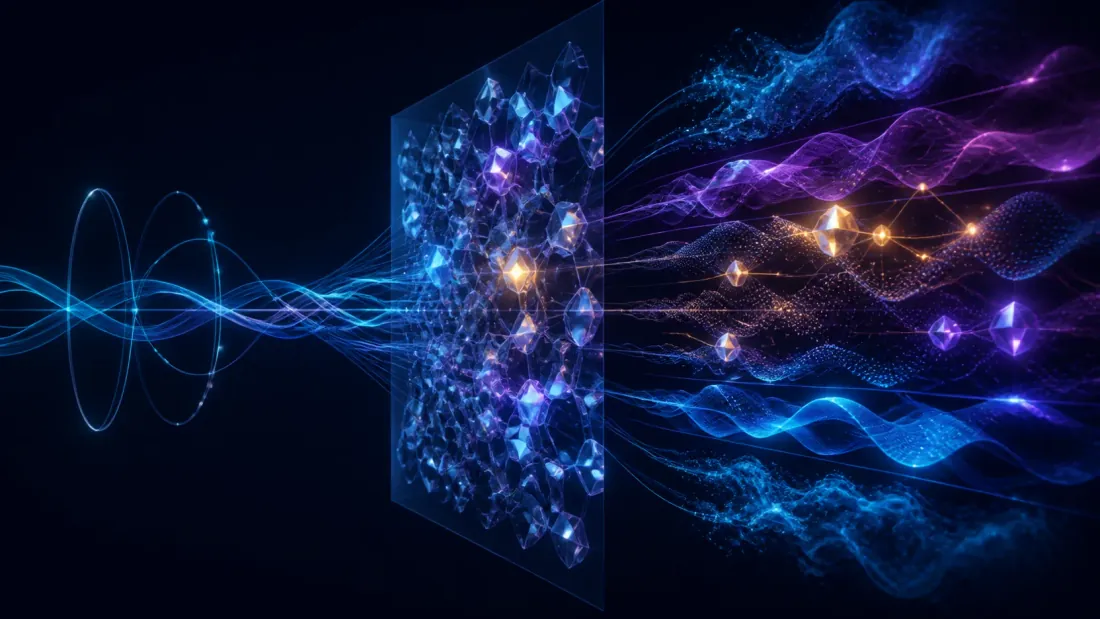
Standard DMD raw state vector पर काम करता है। EDMD पहले data को nonlinear basis functions की dictionary से lift करता है।
Scalar functions की dictionary में functions हों, तो lifted state परिभाषित करें:
EDMD को के साथ खोजता है। नीचे के code में प्रयुक्त convention — states columns के रूप में, बाईं ओर काम करता है:
| Dictionary type | Functions | Captures |
|---|---|---|
| Polynomial | Nonlinear cross-asset interactions | |
| Radial basis (RBF) | Local similarity, regime clustering | |
| Time-delay embedding | Memory / autoregressive structure | |
| Fourier | Known periodicities (intraday, weekly) | |
| Volatility features | Heteroskedasticity, vol clustering |
Dictionary वह जगह है जहां domain knowledge प्रवेश करता है, और time-delay row ही Koopman-specific कारण है कि delay coordinates की परवाह क्यों करें: वे अलग से जोड़ी गई technique नहीं, बल्कि lifting map का एक और block हैं। Embedding स्वयं — delay , embedding dimension और इसके पीछे का reconstruction theorem — पहले ही algorithmic trading के लिए complex manifolds में introduce और code किया गया है; वहां के delay vectors लें और उन्हें सीधे build_financial_dictionary में extra rows की तरह feed करें।
import numpy as np
from itertools import combinations_with_replacement

def build_financial_dictionary(X: np.ndarray, max_poly_degree: int = 2,
                               include_volatility: bool = True,
                               delay_steps: int = 0) -> np.ndarray:
    """
    Build a dictionary of nonlinear observables for EDMD.

    X : np.ndarray, shape (n_features, n_snapshots)
    Returns Z of shape (n_dict, n_snapshots - delay_steps).
    """
    n_features, n_snapshots = X.shape
    offset = max(delay_steps, 0)
    X_eff = X[:, offset:]
    n_eff = X_eff.shape[1]

    lifted = [X_eff]  # degree-1 terms (identity)

    if max_poly_degree >= 2:
        for deg in range(2, max_poly_degree + 1):
            for combo in combinations_with_replacement(range(n_features), deg):
                term = np.ones(n_eff)
                for idx in combo:
                    term *= X_eff[idx]
                lifted.append(term.reshape(1, -1))

    if include_volatility:
        lifted.append(np.abs(X_eff))   # absolute returns
        lifted.append(X_eff ** 2)      # squared returns

    for d in range(1, delay_steps + 1):
        lifted.append(X[:, offset - d : n_snapshots - d])

    return np.vstack(lifted)


def edmd(X: np.ndarray, dictionary_fn=None, reg: float = 1e-8,
         **dict_kwargs) -> tuple:
    """
    Extended Dynamic Mode Decomposition.

    Solves Z1 ~= K @ Z0 in the least-squares sense. Uses a least-squares
    solve rather than an explicit Gram inverse: `inv` on a near-singular
    dictionary Gram matrix is how EDMD spectra get silently corrupted.
    """
    if dictionary_fn is None:
        dictionary_fn = lambda x: build_financial_dictionary(x, **dict_kwargs)

    Z = dictionary_fn(X)
    Z0, Z1 = Z[:, :-1], Z[:, 1:]

    p = Z0.shape[0]
    G = Z0 @ Z0.T + reg * np.eye(p)   # regularised Gram matrix
    A = Z1 @ Z0.T

    K = np.linalg.solve(G, A.T).T

    eigenvalues, eigenvectors = np.linalg.eig(K)
    return K, eigenvalues, eigenvectors
6. Deep Koopman Networks
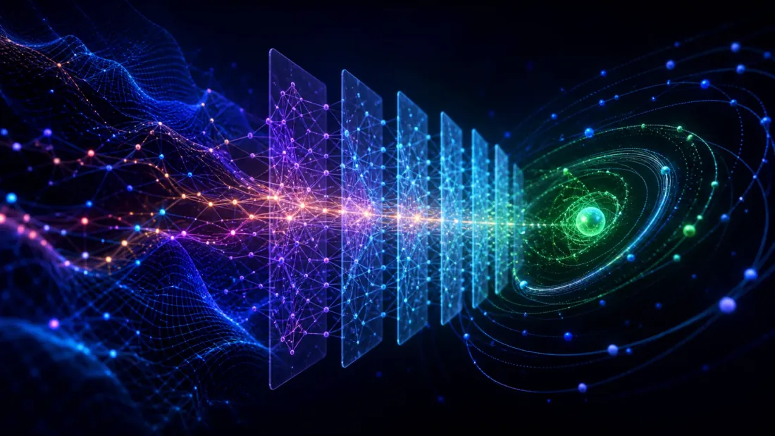
EDMD dictionary hand-crafted है, जो एक वास्तविक limitation है जब Koopman-invariant subspace अज्ञात हो। Deep Koopman networks lifting और operator को संयुक्त रूप से सीखते हैं।
Architecture एक autoencoder है — encoder, latent code, decoder, reconstruction loss, सब कुछ algotrading में anomaly detection में introduce किया गया है — और एक addition है जो इस section का पूरा point है: linearity loss, जो latent dynamics को एक single learned matrix से गुजरने के लिए बाध्य करता है।
x_k  -->  [Encoder φ]  -->  z_k  -->  [Linear K]  -->  z_{k+1}  -->  [Decoder ψ]  -->  x̂_{k+1}
                              |                            |
                              +--- Linearity loss: ‖z_{k+1} - K z_k‖ ---+
term के बिना आपके पास एक ordinary autoencoder है, जिसके latent space के बाद संयोग से matrix multiply होता है। इसके साथ network को ऐसी किसी latent representation के लिए penalise किया जाता है जिसका evolution linear नहीं है — यही learned को Koopman approximation और उसके eigenvalues को section 4 के DMD spectrum के साथ comparable बनाता है।
import torch
import torch.nn as nn

class DeepKoopman(nn.Module):
    """Deep Koopman autoencoder: learned lifting + linear latent dynamics."""

    def __init__(self, input_dim: int, latent_dim: int, hidden_dim: int = 128):
        super().__init__()

        self.encoder = nn.Sequential(
            nn.Linear(input_dim, hidden_dim), nn.ReLU(),
            nn.Linear(hidden_dim, hidden_dim), nn.ReLU(),
            nn.Linear(hidden_dim, latent_dim),
        )
        self.decoder = nn.Sequential(
            nn.Linear(latent_dim, hidden_dim), nn.ReLU(),
            nn.Linear(hidden_dim, hidden_dim), nn.ReLU(),
            nn.Linear(hidden_dim, input_dim),
        )
        self.K = nn.Linear(latent_dim, latent_dim, bias=False)

    def encode(self, x: torch.Tensor) -> torch.Tensor:
        return self.encoder(x)

    def decode(self, z: torch.Tensor) -> torch.Tensor:
        return self.decoder(z)

    def forward(self, x_k: torch.Tensor) -> dict:
        z_k = self.encode(x_k)
        z_k1_pred = self.K(z_k)
        return {
            "z_k": z_k,
            "z_k1_pred": z_k1_pred,
            "x_k1_pred": self.decode(z_k1_pred),
            "x_k_recon": self.decode(z_k),
        }

    def multi_step_predict(self, x_0: torch.Tensor, n_steps: int) -> torch.Tensor:
        """Roll out by repeated application of the linear operator."""
        z = self.encode(x_0)
        preds = []
        for _ in range(n_steps):
            z = self.K(z)
            preds.append(self.decode(z))
        return torch.stack(preds, dim=1)

    def latent_spectrum(self) -> np.ndarray:
        """Eigenvalues of the learned K — directly comparable to DMD's."""
        return np.linalg.eigvals(self.K.weight.detach().cpu().numpy())


def koopman_loss(model: DeepKoopman, x_k: torch.Tensor, x_k1: torch.Tensor,
                 alpha: float = 1.0, beta: float = 0.5) -> torch.Tensor:
    out = model(x_k)
    z_k1_true = model.encode(x_k1)

    prediction = nn.functional.mse_loss(out["x_k1_pred"], x_k1)
    linearity = nn.functional.mse_loss(out["z_k1_pred"], z_k1_true)
    reconstruction = nn.functional.mse_loss(out["x_k_recon"], x_k)

    return prediction + alpha * linearity + beta * reconstruction
latent_spectrum ही इस model को sequence model अपनाने के बजाय train करने का कारण है: learned operator अभी भी एक matrix है, इसलिए section 4.2 का stability test और section 4.3 का lead-lag test deep model पर भी बिना बदलाव लागू होते हैं।
7. Practical Considerations और Pitfalls
Rank selection. Truncation rank bias-variance dial है — बहुत कम dynamics miss करता है, बहुत अधिक noise fit करता है। Singular-value elbow को आंख से तय न करें; blog पहले ही vectors और matrices के साथ complex arbitrage में Random Matrix Theory के Marchenko-Pastur bound के साथ "noise fit करने से पहले कितने components" का सही उत्तर देता है। अपने window shape के लिए जिन components की singular values Marchenko-Pastur edge से अधिक हों, उन्हें रखें और प्रकाशित हर spectrum के साथ परिणामी स्पष्ट रूप से बताएं।
Window length. Koopman theory fixed मानती है; markets ऐसा कोई map नहीं देते। Rolling refits अनिवार्य हैं, और section 4.2 की stability curve ठीक यही diagnostic है कि चुनी गई window estimation के लिए पर्याप्त लंबी और एक regime के भीतर रहने के लिए पर्याप्त छोटी है या नहीं।
Noise sensitivity. Financial data का signal-to-noise ratio कम होता है और standard DMD में noise से biased होता है। Modes unstable हैं यह निष्कर्ष निकालने से पहले आजमाने योग्य remedies:
- Total DMD (TDMD) — total least squares के माध्यम से और दोनों को noisy मानता है।
- Optimized DMD — eigenvalue-mode decomposition को residual Frobenius norm के विरुद्ध सीधे optimize करता है।
- Kernel EDMD — dictionary बनाए बिना implicitly high-dimensional feature space में काम करता है।
यदि TDMD के अंतर्गत mode stability materially बढ़ती है, तो instability measurement noise थी। यदि नहीं बढ़ती, तो वह market था।
8. DMD कहां बैठता है

| Method | Linearity | Interpretable | Multi-step forecast |
|---|---|---|---|
| DMD | Linear in state space | Yes (modes + eigenvalues) | Stable (matrix power) |
| EDMD | Linear in lifted space | Yes, given the dictionary | Stable (matrix power) |
| Deep Koopman | Linear in learned space | Moderate (inspect latent K) | Stable (matrix power) |
Volatility-specific forecasting के लिए comparison point GARCH family है — crypto के लिए GARCH volatility forecasting देखें। Fully nonlinear sequence models और उनके interpretability तथा error-accumulation trade-offs के लिए trading में Temporal Fusion Transformer देखें।
DMD का niche संकरा लेकिन वास्तविक है: autoregressive rollout के बजाय single matrix power से generated multi-step forecasts, जिसमें हर mode inspectable है। क्या इस niche में alpha है, यह section 4 का सवाल है, इस table का नहीं।
Conclusion

Koopman theory market dynamics को देखने का सचमुच elegant तरीका है, और elegance ही कारण है कि इसे उपलब्ध सबसे कठोर test की जरूरत है। मुख्य बातें:
- DMD fit करें, फिर तुरंत fit को test करें। Adjacent windows का subspace overlap, phase-randomised null के विरुद्ध मापा गया, एक दोपहर में बता देता है कि आपने structure खोजा है या एक window को याद किया है।
- Rolling spectral radius monitor करने योग्य एक scalar है, और उसका मूल्य पूरी तरह lead-lag result पर निर्भर करता है। Lag 0 पर यह volatility proxy है; negative lag पर regime warning है।
- Amplitudes को last snapshot पर anchor करें और eigenvalues को कभी window length तक power न दें। वास्तविक दुनिया में DMD के बहुत से "signals" floating-point artifacts हैं।
- Rank को Marchenko-Pastur से चुनें, elbow को आंख से देखकर नहीं, और हर spectrum के साथ rank publish करें।
- Spectrum plot result नहीं है। इसके ऊपर बनाई गई कोई भी strategy fees, slippage और deflated Sharpe test से बचने के बाद ही गिनी जाएगी।
इनसे आगे के implementations के लिए PyDMD library DMD variants को व्यापक रूप से cover करती है, और Mallen et al. का reference code deep Koopman पक्ष को cover करता है।
Markets messy, non-stationary और partially observed बने रहेंगे। Koopman theory उस mess से structure निकालने का principled lens देती है — बशर्ते आप जांचें कि वह structure अगले सप्ताह भी मौजूद है।
References और आगे पढ़ना:
- B. O. Koopman, "Hamiltonian Systems and Transformation in Hilbert Space," Proceedings of the National Academy of Sciences, 1931.
- J. H. Tu et al., "On Dynamic Mode Decomposition: Theory and Applications," Journal of Computational Dynamics, 2014.
- M. O. Williams, I. G. Kevrekidis, C. W. Rowley, "A Data-Driven Approximation of the Koopman Operator: Extending Dynamic Mode Decomposition," Journal of Nonlinear Science, 2015.
- B. Lusch, J. N. Kutz, S. L. Brunton, "Deep Learning for Universal Linear Embeddings of Nonlinear Dynamics," Nature Communications, 2018.
- J. Mann and J. N. Kutz, "Dynamic Mode Decomposition for Financial Trading Strategies," Quantitative Finance, 2016.
- A. Mallen et al., "Koopman Neural Forecaster for Time Series with Temporal Distribution Shifts," ICML, 2023.
- E. Gonzalez and M. Generelo, "Analysis of chaotic economic models through Koopman operators, EDMD, Takens' theorem and Machine Learning," Data Science in Finance and Economics, 2022.
Authors
Trading-systems engineer
Trading-systems engineer building bots since 2017: cross-exchange arbitrage (connected up to 30 venues), cointegration-based pairs arbitrage across spot and futures, scalping, news and sentiment-driven strategies, trend algorithms, and portfolio management and balancing algorithms. Also builds sub-millisecond order execution, big-data warehouses, backtesting engines, AI agents, and trading interfaces (incl. open-source profitmaker.cc). Stack: JS/TS, Python, Rust/Zig/Go, DevOps, backend, frontend, architecture.
Read More

XGBoost for Return Direction: Class Imbalance and Decision Thresholds

Irregular Time in Tick Models: Continuous-Time Encodings vs. Plain Positional Embeddings