Koopman Operators and DMD: Do Market Modes Survive Out-of-Sample?

Dynamic Mode Decomposition ให้สเปกตรัมของ eigenvalue เชิงซ้อนจำนวนหนึ่ง โดยแต่ละตัวมีอัตราการเติบโตและความถี่ และผูกกับโหมดเชิงพื้นที่ของสินทรัพย์ทั้งหมดของคุณ มันดูเหมือนโครงสร้าง คำถามสำคัญคือมัน เป็น โครงสร้างจริงหรือเป็นเพียงตัวดำเนินการเชิงเส้นที่จดจำ noise ของหน้าต่างเดียว
คำถามนี้แบ่งเป็นสองส่วนที่ทดสอบได้ และบทความนี้สร้างขึ้นรอบสองส่วนนั้น:
- ความคงอยู่ของโหมด fit DMD บนหน้าต่าง และ โหมดเด่นครอบคลุม subspace เดียวกันหรือสลับไปมาทุกครั้งที่ refit? หากสลับ DMD ก็เป็นเพียงการแยกแบบ in-sample — การพูดอย่างตรงไปตรงมามีประโยชน์กว่าบทสอนอีกหนึ่งบท
- รัศมีสเปกตรัมเป็นตัวชี้นำ modulus ของ eigenvalue ที่ใหญ่ที่สุด เป็นสเกลาร์เดียวที่สรุปว่าพลวัตที่ fit มีความรุนแรงเพียงใด มัน นำหน้า ความผันผวนจริง ล้าหลัง หรือเพียงบอกสิ่งเดิม? ทุกคำตอบเผยแพร่ได้ แต่มีเพียงคำตอบแรกที่นำไปเทรดได้
ที่ตลาดเป็นระบบไม่เชิงเส้นและไม่อยู่กับที่ถือเป็นสมมติฐานที่นี่ ไม่ใช่ประเด็นที่ต้องพิสูจน์ — บล็อกได้อธิบายแล้วด้วยเรขาคณิต phase-space ใน attractors in algotrading และสถิติ BTC ราย regime ที่วัดจริงใน การตรวจจับ regime ด้วย HMM ต่อไปคือคำถามที่แคบลงว่า non-stationarity ส่งผลอย่างไรต่อ ตัวดำเนินการ Koopman ที่ fit แล้ว และจะวัดอย่างไร
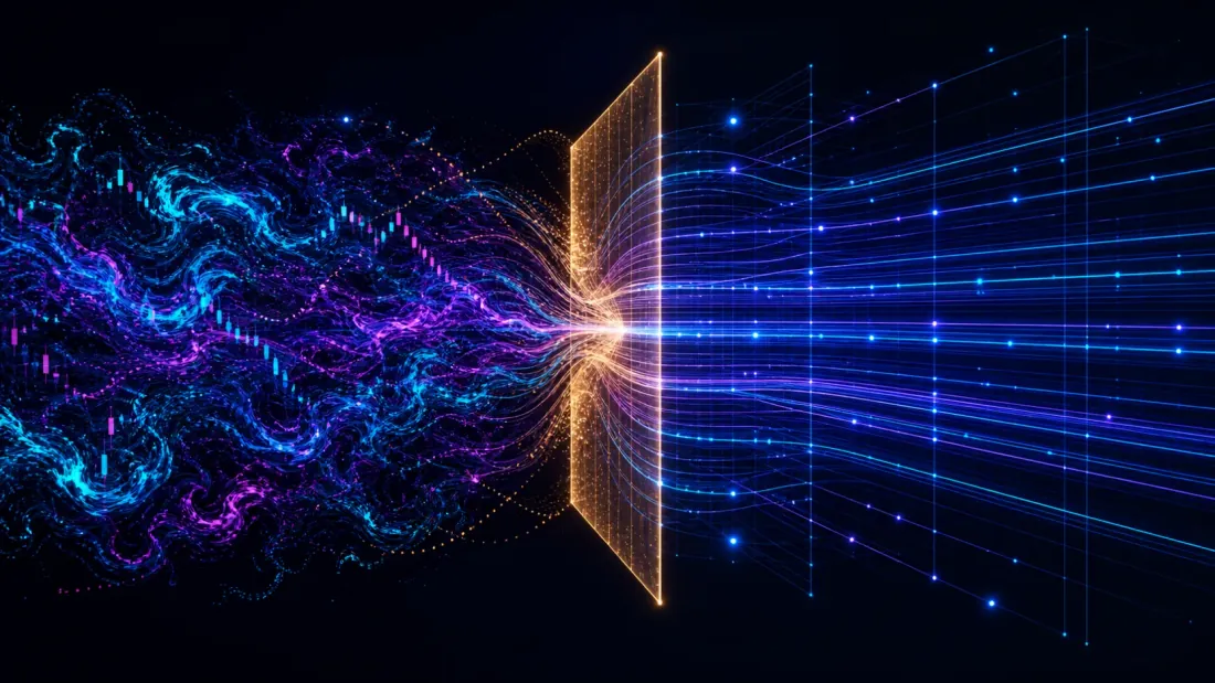
1. แนวคิดหลัก: ทำให้พลวัตไม่เชิงเส้นเป็นเชิงเส้น
พิจารณาระบบพลวัตเวลาไม่ต่อเนื่องบนปริภูมิสถานะ :
โดย เป็น mapping ที่อาจไม่เชิงเส้น สำหรับตลาด คือเวกเตอร์ของผลตอบแทนสินทรัพย์ ความผันผวน หรือ imbalance ของ order book ในขั้นเวลา
ตัวดำเนินการ Koopman ไม่ได้ทำงานกับสถานะ โดยตรง แต่ทำงานกับ ฟังก์ชัน observable ค่า scalar :
คุณสมบัติสำคัญคือ เป็นเชิงเส้น แม้ จะไม่เชิงเส้น ราคาที่ต้องจ่ายคือ dimensionality — ทำงานใน function space มิติอนันต์ การประมาณมิติจำกัดที่ดีให้ความสามารถของพลวัตไม่เชิงเส้นพร้อมความจัดการง่ายของพีชคณิตเชิงเส้น: prediction กลายเป็นการยกกำลังเมทริกซ์ และตรวจสอบทุกโหมดได้แทนที่จะซ่อนอยู่ในน้ำหนักเครือข่าย
2. การแยกเชิงสเปกตรัมของตัวดำเนินการ Koopman

หาก มี eigenvalue และ eigenfunction จะได้ และ observable ใด ๆ ใน span ของ eigenfunction เหล่านี้จะแยกได้เป็น:
โดย คือ โหมด Koopman — สัมประสิทธิ์แบบเวกเตอร์ที่อธิบายว่า eigenfunction แต่ละตัวมีส่วนต่อ observable vector ทั้งหมดอย่างไร
eigenvalue แต่ละตัว เข้ารหัสอัตราการเติบโตหรือ decay () และความถี่การสั่น ():
| Component | Eigenvalue property | Financial interpretation |
|---|---|---|
| Trend | , | Slow drift, momentum |
| Cycles | , | Oscillations, seasonality |
| Transients | Decaying shocks, short-lived moves | |
| Unstable modes | Growing, explosive dynamics |
ตารางนี้คือคำสัญญา ส่วนที่ 4 คือจุดที่ตรวจสอบคำสัญญากับข้อมูล
3. Dynamic Mode Decomposition (DMD)
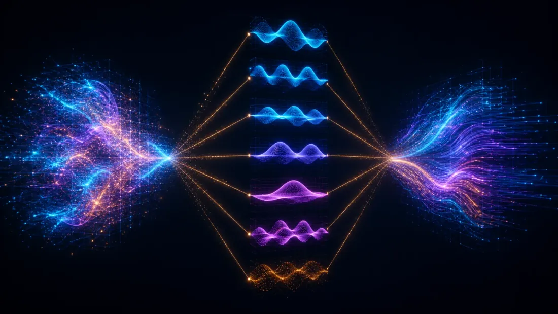
DMD คืออัลกอริทึมหลักสำหรับประมาณ จากข้อมูล เมื่อจัด snapshot เป็นเมทริกซ์:
DMD ค้นหาตัวดำเนินการเชิงเส้น ที่ fit ได้ดีที่สุด โดยมี :
- คำนวณ SVD:
- โปรเจกต์:
- ทำ eigendecomposition:
- กู้คืนโหมดในปริภูมิเต็ม:
คอลัมน์ของ คือ โหมด DMD และแนวทแยงของ เก็บ eigenvalue ของ DMD
import numpy as np
from numpy.linalg import svd, eig, lstsq

def dmd(X: np.ndarray, rank: int | None = None) -> tuple:
    """
    Dynamic Mode Decomposition.

    Parameters
    ----------
    X : np.ndarray, shape (n_features, n_snapshots)
        Data matrix where each column is a state snapshot.
    rank : int or None
        Truncation rank for the SVD. None = no truncation.

    Returns
    -------
    eigenvalues : np.ndarray, shape (r,)
        DMD eigenvalues (approximating Koopman eigenvalues).
    modes : np.ndarray, shape (n_features, r)
        DMD modes (columns), L2-normalised.
    amplitudes : np.ndarray, shape (r,)
        Mode amplitudes fitted to the FINAL snapshot, so that a one-step
        forecast is simply modes @ (eigenvalues * amplitudes).
    """
    X0 = X[:, :-1]
    X1 = X[:, 1:]

    U, S, Vh = svd(X0, full_matrices=False)

    if rank is not None:
        U = U[:, :rank]
        S = S[:rank]
        Vh = Vh[:rank, :]

    S_inv = np.diag(1.0 / S)

    A_tilde = U.conj().T @ X1 @ Vh.conj().T @ S_inv
    eigenvalues, W = eig(A_tilde)

    modes = X1 @ Vh.conj().T @ S_inv @ W

    norms = np.linalg.norm(modes, axis=0)
    norms[norms == 0] = 1.0
    modes = modes / norms

    amplitudes = lstsq(modes, X[:, -1].astype(complex), rcond=None)[0]

    return eigenvalues, modes, amplitudes
มีตัวเลือกที่ตั้งใจสองอย่าง โหมดถูก ทำให้เป็น L2-normalised เพราะส่วน 4.2 เปรียบเทียบ subspace ของโหมดระหว่างหน้าต่าง และ amplitude ที่ไม่ normalize จะกลบการเปรียบเทียบ Amplitude fit กับ snapshot สุดท้าย ไม่ใช่ตัวแรก ดังนั้น forecast จะไม่ยก eigenvalue เป็นกำลังสูง ซึ่งเป็นต้นเหตุของ numerical blow-up ที่ทำให้สัญญาณ DMD แบบ naїve ดูเหมือนพลวัตทั้งที่เป็น floating-point overflow
4. การวัดผล
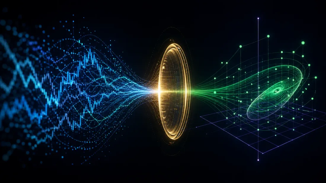
นี่คือส่วนที่ไม่ใช่เนื้อหาแบบ textbook ทุกอย่างข้างต้นเป็นขั้นตอน fitting ส่วนถัดไปคือ protocol เพื่อดูว่า fit มีความหมายจริงหรือไม่
ข้อมูล ใช้ข้อมูล exchange ของโครงการเอง — cross-section ของ BTC, ETH และ alt ที่มีสภาพคล่องบน grid นาทีหรือ tick ที่สม่ำเสมอ ไม่ใช่การดาวน์โหลด ETF หุ้นรายวัน บล็อกนี้เน้น crypto และเหตุผลด้าน microstructure ไม่สามารถย้ายมาใช้ตรง ๆ ได้ สร้าง โดยให้สินทรัพย์อยู่ในแถวและเวลาอยู่ในคอลัมน์ ใช้ log return ที่หักค่าเฉลี่ยรายสินทรัพย์ในแต่ละหน้าต่าง
4.1 สเปกตรัม eigenvalue
สำหรับหน้าต่างตัวแทน ให้รายงานว่า eigenvalue ตัวมีกี่ตัวอยู่ใน tolerance ของวงกลมหน่วย แต่ละตัวสอดคล้องกับคาบการสั่น เป็นชั่วโมง เท่าใด (period bars แล้วแปลงหน่วย) และโหมด อันดับแรก reconstruct variance ของ return ได้กี่ส่วน
def spectrum_report(eigenvalues: np.ndarray, bar_minutes: float,
                    tol: float = 0.05) -> list[dict]:
    """
    Turn a DMD spectrum into human-readable rows: modulus, period in hours,
    and whether the eigenvalue sits on the unit circle within `tol`.
    """
    rows = []
    for lam in eigenvalues:
        modulus = float(np.abs(lam))
        omega = float(np.angle(lam))
        period_hours = (2 * np.pi / abs(omega)) * bar_minutes / 60 if omega else np.inf
        rows.append({
            "modulus": modulus,
            "period_hours": period_hours,
            "on_unit_circle": abs(modulus - 1.0) < tol,
            "regime": "unstable" if modulus > 1 + tol
                      else "persistent" if abs(modulus - 1.0) <= tol
                      else "decaying",
        })
    return sorted(rows, key=lambda r: -r["modulus"])


def reconstruction_r2(X: np.ndarray, modes: np.ndarray,
                      eigenvalues: np.ndarray, amplitudes: np.ndarray) -> float:
    """Fraction of in-window return variance captured by the truncated modes."""
    n_steps = X.shape[1]
    powers = eigenvalues[:, None] ** np.arange(-(n_steps - 1), 1)
    X_hat = (modes @ (amplitudes[:, None] * powers)).real
    resid = np.var(X - X_hat)
    return 1.0 - resid / np.var(X)
รายงานสเปกตรัมอย่างซื่อสัตย์ก็มีค่าพอเป็นบทความแล้ว หากไม่มีอะไรอยู่ใกล้วงกลมหน่วย ก็ไม่มีวัฏจักรถาวรให้เทรด และเรื่อง "seasonality รายปี" จากวรรณกรรมหุ้นก็ใช้กับ crypto 24/7 ไม่ได้
4.2 ความเสถียรของโหมดระหว่างหน้าต่างที่ติดกัน
การทดสอบชี้ขาดคือ fit DMD บนหน้าต่าง แล้วบน และวัดว่า subspace ของโหมดเด่นยังเหลืออยู่เท่าใด สถิติที่ถูกต้องไม่ใช่ correlation แบบ naїve ของ mode vector — ลำดับโหมดและ complex phase เป็นสิ่ง arbitrary — แต่คือ principal angles ระหว่างสอง subspace
def subspace_stability(modes_a: np.ndarray, modes_b: np.ndarray,
                       k: int = 3) -> float:
    """
    Overlap between the leading-k DMD mode subspaces of two adjacent windows.

    Returns the mean cosine of the principal angles: 1.0 = identical subspace,
    0.0 = orthogonal. Immune to mode reordering and complex phase, both of
    which are arbitrary in a DMD fit.
    """
    Qa, _ = np.linalg.qr(modes_a[:, :k])
    Qb, _ = np.linalg.qr(modes_b[:, :k])
    sing = np.linalg.svd(Qa.conj().T @ Qb, compute_uv=False)
    return float(np.mean(np.clip(sing, 0.0, 1.0)))


def stability_curve(returns: np.ndarray, window: int, step: int,
                    rank: int, k: int = 3) -> np.ndarray:
    """Subspace overlap between every pair of adjacent windows."""
    fits = []
    for t_end in range(window, returns.shape[1], step):
        evals, modes, _ = dmd(returns[:, t_end - window:t_end], rank=rank)
        order = np.argsort(-np.abs(evals))
        fits.append(modes[:, order])
    return np.array([subspace_stability(fits[i], fits[i + 1], k=k)
                     for i in range(len(fits) - 1)])
รายงานการกระจายของ overlap นี้และเปรียบเทียบกับ null โดยคำนวณสถิติเดียวกันบน surrogate ที่สุ่มเฟสของ return เดียวกัน หาก overlap สูงแต่ไม่สูงกว่า surrogate null แสดงว่าโหมดกำลังติดตามโครงสร้าง covariance ไม่ใช่พลวัต
4.3 รัศมีสเปกตรัมแบบเลื่อนเทียบกับความผันผวนที่เกิดขึ้นจริง
ข้ออ้างที่ต้องทดสอบคือ ที่คำนวณใหม่บน rolling windows เคลื่อนที่ ก่อน realized volatility ไม่ใช่พร้อมกัน สเกลาร์นี้ใหม่ในเชิงกลไก — บล็อกเคยติดตาม geometric scalars แบบ real time โดยเฉพาะ Kobayashi curvature ใน complex manifolds for algorithmic trading — แต่ modulus ของ Koopman eigenvalue เป็นปริมาณต่างชนิดที่มี failure mode ต่างกัน จึงควรมี lead-lag test ของตัวเอง ไม่ใช่ใช้ pitch เดิม
def rolling_spectral_radius(returns: np.ndarray, window: int = 1440,
                            step: int = 60, rank: int = 5) -> dict:
    """
    Rolling DMD spectrum for regime monitoring.

    returns : np.ndarray, shape (n_assets, n_timesteps)
    window  : rolling window length in bars
    step    : bars between refits
    """
    idx, radii, dom_freq = [], [], []

    for t_end in range(window, returns.shape[1], step):
        X_win = returns[:, t_end - window:t_end]
        try:
            evals, _, _ = dmd(X_win, rank=rank)
        except np.linalg.LinAlgError:
            continue

        idx.append(t_end)
        radii.append(float(np.max(np.abs(evals))))

        on_circle = np.abs(np.abs(evals) - 1.0) < 0.1
        if on_circle.any():
            sel = evals[on_circle]
            dom_freq.append(float(np.abs(np.angle(sel[np.argmax(np.abs(sel))])) / (2 * np.pi)))
        else:
            dom_freq.append(0.0)

    return {"index": np.array(idx),
            "spectral_radius": np.array(radii),
            "dominant_frequency": np.array(dom_freq)}


def lead_lag(signal: np.ndarray, target: np.ndarray, max_lag: int = 24) -> dict:
    """
    Cross-correlation of `signal` against `target` over +/- max_lag steps.
    A peak at negative lag means the signal LEADS the target.
    """
    s = (signal - signal.mean()) / (signal.std() + 1e-12)
    y = (target - target.mean()) / (target.std() + 1e-12)
    lags = np.arange(-max_lag, max_lag + 1)
    corrs = []
    for L in lags:
        if L < 0:
            corrs.append(float(np.corrcoef(s[:L], y[-L:])[0, 1]))
        elif L > 0:
            corrs.append(float(np.corrcoef(s[L:], y[:-L])[0, 1]))
        else:
            corrs.append(float(np.corrcoef(s, y)[0, 1]))
    corrs = np.array(corrs)
    return {"lags": lags, "corr": corrs, "peak_lag": int(lags[np.argmax(np.abs(corrs))])}
จัดแนว spectral_radius กับ realized volatility ที่คำนวณบน grid เดียวกันแล้วอ่าน peak_lag หาก peak อยู่ที่ lag 0 แปลว่า เป็นเพียงการกล่าวถึง volatility ซ้ำพร้อมขั้นตอนเพิ่ม หาก peak อยู่ที่ lag ลบและเสถียรตลอด sample และ rank นั่นคือเวอร์ชันเดียวของบทความที่มีข้ออ้างนำไปเทรดได้
หมายเหตุเกี่ยวกับสิ่งที่จะทำหลังได้ผลลัพธ์เป็นบวก
หาก นำหน้า ขั้นตอนถัดไปที่ชัดเจนคือการสร้าง cross-sectional: จัดอันดับสินทรัพย์ตาม return ขั้นถัดไปที่ DMD พยากรณ์ แล้ว long ผู้ชนะและ short ผู้แพ้ตามคำทำนาย โครงสร้างนี้ไม่ใช่เรื่องใหม่ — เป็น factor-residual trade ที่กล่าวถึงแล้วใน statistical arbitrage and pairs trading in crypto และส่วนที่ 4 ของ complex arbitrage with vectors and matrices; จุดเฉพาะของ Koopman คือ eigenportfolio มี eigenvalue ที่เปลี่ยนตามเวลาแทน loading ของ PCA แบบคงที่
ส่วนกลยุทธ์ถูกละไว้โดยตั้งใจ เพราะยังไม่ได้ backtest ที่นี่พร้อมค่าธรรมเนียมและ slippage เมื่อทำแล้วต้องผ่านมาตรฐานของบล็อกเอง คือ significance test ใน Deflated Sharpe Ratio และ multiple testing เทียบกับตัวอย่างโต้แย้งอย่าง ผลลบอย่างซื่อสัตย์ กราฟสเปกตรัม DMD ไม่ใช่ผลลัพธ์
สำหรับ one-step forecast implementation ที่ถูกต้องต้องพยากรณ์จาก snapshot สุดท้าย ไม่ใช่เผยแพร่ eigenvalue ด้วยกำลังเท่าความยาวหน้าต่าง:
def dmd_one_step(returns: np.ndarray, rank: int = 4) -> np.ndarray:
    """
    One-step-ahead prediction from the final snapshot of the window.

    Never raise eigenvalues to the window length: any |lambda| != 1 then
    overflows or underflows and the "signal" becomes numerical garbage.
    """
    evals, modes, amplitudes = dmd(returns, rank=rank)
    return (modes @ (evals * amplitudes)).real
5. Extended DMD (EDMD): observable ไม่เชิงเส้น

DMD มาตรฐานทำงานกับ raw state vector ส่วน EDMD จะยกข้อมูลผ่าน dictionary ของ basis functions ไม่เชิงเส้นก่อน
เมื่อมี dictionary ของฟังก์ชัน scalar ให้กำหนด lifted state ดังนี้:
EDMD ค้นหา ที่มี ตาม convention ของโค้ดด้านล่าง — state เป็น คอลัมน์ และ ทำงานทางซ้าย:
| Dictionary type | Functions | Captures |
|---|---|---|
| Polynomial | Nonlinear cross-asset interactions | |
| Radial basis (RBF) | Local similarity, regime clustering | |
| Time-delay embedding | Memory / autoregressive structure | |
| Fourier | Known periodicities (intraday, weekly) | |
| Volatility features | Heteroskedasticity, vol clustering |
Dictionary คือจุดที่ความรู้โดเมนเข้ามา และแถว time-delay คือเหตุผลเฉพาะของ Koopman ที่ต้องสนใจ delay coordinates: มันไม่ใช่เทคนิคแยกที่นำมาต่อเพิ่ม แต่เป็นอีกบล็อกหนึ่งของ lifting map ตัว embedding เอง — การเลือก delay , embedding dimension และ reconstruction theorem — ถูกแนะนำและเขียนโค้ดไว้แล้วใน complex manifolds for algorithmic trading; นำ delay vectors จากที่นั่นส่งตรงเข้า build_financial_dictionary เป็นแถวเพิ่ม
import numpy as np
from itertools import combinations_with_replacement

def build_financial_dictionary(X: np.ndarray, max_poly_degree: int = 2,
                               include_volatility: bool = True,
                               delay_steps: int = 0) -> np.ndarray:
    """
    Build a dictionary of nonlinear observables for EDMD.

    X : np.ndarray, shape (n_features, n_snapshots)
    Returns Z of shape (n_dict, n_snapshots - delay_steps).
    """
    n_features, n_snapshots = X.shape
    offset = max(delay_steps, 0)
    X_eff = X[:, offset:]
    n_eff = X_eff.shape[1]

    lifted = [X_eff]  # degree-1 terms (identity)

    if max_poly_degree >= 2:
        for deg in range(2, max_poly_degree + 1):
            for combo in combinations_with_replacement(range(n_features), deg):
                term = np.ones(n_eff)
                for idx in combo:
                    term *= X_eff[idx]
                lifted.append(term.reshape(1, -1))

    if include_volatility:
        lifted.append(np.abs(X_eff))   # absolute returns
        lifted.append(X_eff ** 2)      # squared returns

    for d in range(1, delay_steps + 1):
        lifted.append(X[:, offset - d : n_snapshots - d])

    return np.vstack(lifted)


def edmd(X: np.ndarray, dictionary_fn=None, reg: float = 1e-8,
         **dict_kwargs) -> tuple:
    """
    Extended Dynamic Mode Decomposition.

    Solves Z1 ~= K @ Z0 in the least-squares sense. Uses a least-squares
    solve rather than an explicit Gram inverse: `inv` on a near-singular
    dictionary Gram matrix is how EDMD spectra get silently corrupted.
    """
    if dictionary_fn is None:
        dictionary_fn = lambda x: build_financial_dictionary(x, **dict_kwargs)

    Z = dictionary_fn(X)
    Z0, Z1 = Z[:, :-1], Z[:, 1:]

    p = Z0.shape[0]
    G = Z0 @ Z0.T + reg * np.eye(p)   # regularised Gram matrix
    A = Z1 @ Z0.T

    K = np.linalg.solve(G, A.T).T

    eigenvalues, eigenvectors = np.linalg.eig(K)
    return K, eigenvalues, eigenvectors
6. Deep Koopman Networks

Dictionary EDMD dibuat secara manual, yang menjadi keterbatasan nyata ketika subspace invariant Koopman tidak diketahui Deep Koopman networks mempelajari lifting dan operator secara bersama
Arsitekturnya adalah autoencoder — encoder, latent code, decoder dan reconstruction loss seperti diperkenalkan dalam anomaly detection in algotrading — dengan tambahan yang menjadi inti bagian ini: linearity loss yang memaksa dinamika laten melewati satu matriks yang dipelajari
x_k  -->  [Encoder φ]  -->  z_k  -->  [Linear K]  -->  z_{k+1}  -->  [Decoder ψ]  -->  x̂_{k+1}
                              |                            |
                              +--- Linearity loss: ‖z_{k+1} - K z_k‖ ---+
Tanpa suku , Anda memiliki autoencoder biasa yang ruang latennya kebetulan diikuti perkalian matriks Dengan suku ini, jaringan mendapat penalti untuk representasi laten yang evolusinya tidak linear — inilah yang membuat menjadi aproksimasi Koopman dan eigenvalue-nya dapat dibandingkan dengan spektrum DMD bagian 4
import torch
import torch.nn as nn

class DeepKoopman(nn.Module):
    """Deep Koopman autoencoder: learned lifting + linear latent dynamics."""

    def __init__(self, input_dim: int, latent_dim: int, hidden_dim: int = 128):
        super().__init__()

        self.encoder = nn.Sequential(
            nn.Linear(input_dim, hidden_dim), nn.ReLU(),
            nn.Linear(hidden_dim, hidden_dim), nn.ReLU(),
            nn.Linear(hidden_dim, latent_dim),
        )
        self.decoder = nn.Sequential(
            nn.Linear(latent_dim, hidden_dim), nn.ReLU(),
            nn.Linear(hidden_dim, hidden_dim), nn.ReLU(),
            nn.Linear(hidden_dim, input_dim),
        )
        self.K = nn.Linear(latent_dim, latent_dim, bias=False)

    def encode(self, x: torch.Tensor) -> torch.Tensor:
        return self.encoder(x)

    def decode(self, z: torch.Tensor) -> torch.Tensor:
        return self.decoder(z)

    def forward(self, x_k: torch.Tensor) -> dict:
        z_k = self.encode(x_k)
        z_k1_pred = self.K(z_k)
        return {
            "z_k": z_k,
            "z_k1_pred": z_k1_pred,
            "x_k1_pred": self.decode(z_k1_pred),
            "x_k_recon": self.decode(z_k),
        }

    def multi_step_predict(self, x_0: torch.Tensor, n_steps: int) -> torch.Tensor:
        """Roll out by repeated application of the linear operator."""
        z = self.encode(x_0)
        preds = []
        for _ in range(n_steps):
            z = self.K(z)
            preds.append(self.decode(z))
        return torch.stack(preds, dim=1)

    def latent_spectrum(self) -> np.ndarray:
        """Eigenvalues of the learned K — directly comparable to DMD's."""
        return np.linalg.eigvals(self.K.weight.detach().cpu().numpy())


def koopman_loss(model: DeepKoopman, x_k: torch.Tensor, x_k1: torch.Tensor,
                 alpha: float = 1.0, beta: float = 0.5) -> torch.Tensor:
    out = model(x_k)
    z_k1_true = model.encode(x_k1)

    prediction = nn.functional.mse_loss(out["x_k1_pred"], x_k1)
    linearity = nn.functional.mse_loss(out["z_k1_pred"], z_k1_true)
    reconstruction = nn.functional.mse_loss(out["x_k_recon"], x_k)

    return prediction + alpha * linearity + beta * reconstruction
latent_spectrum คือเหตุผลที่ควร train สิ่งนี้แทนการใช้ sequence model: operator ที่เรียนรู้ยังเป็นเมทริกซ์ ดังนั้น stability test ในส่วน 4.2 และ lead-lag test ในส่วน 4.3 จึงใช้กับ deep model ได้โดยไม่เปลี่ยนแปลง
7. ข้อพิจารณาเชิงปฏิบัติและกับดัก
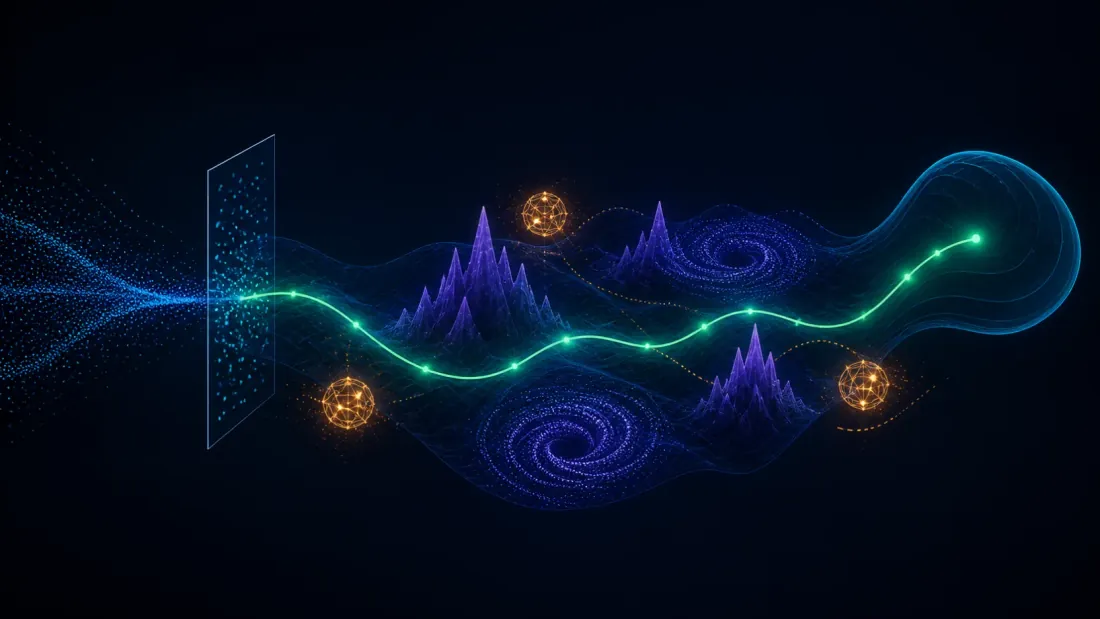
การเลือก rank Rank truncation คือปุ่มปรับ bias-variance — ต่ำเกินไปจะพลาดพลวัต สูงเกินไปจะ fit noise อย่าดู elbow ของ singular-value ด้วยตา บล็อกอธิบายอย่างถูกต้องแล้วว่า "มีกี่ component ก่อนจะ fit noise" ด้วยขอบเขต Marchenko-Pastur จาก Random Matrix Theory ใน complex arbitrage with vectors and matrices เก็บ component ที่ singular value สูงกว่าขอบ Marchenko-Pastur สำหรับรูปแบบหน้าต่าง และระบุ อย่างชัดเจนข้างสเปกตรัมทุกชุดที่เผยแพร่
ความยาวหน้าต่าง ทฤษฎี Koopman สมมติว่า คงที่ แต่ตลาดไม่ได้ให้สิ่งนั้นมา การ rolling refit จึงจำเป็น และ stability curve ในส่วน 4.2 คือ diagnostic โดยตรงว่าหน้าต่างยาวพอสำหรับการ estimate และสั้นพอที่จะอยู่ใน regime เดียวหรือไม่
ความไวต่อ noise ข้อมูลการเงินมี signal-to-noise ratio ต่ำ และ DMD มาตรฐานมี bias จาก noise ใน ควรลองวิธีแก้ต่อไปนี้ก่อนสรุปว่าโหมดไม่เสถียร:
- Total DMD (TDMD) — treats both and as noisy via total least squares.
- Optimized DMD — directly optimises the eigenvalue-mode decomposition against the residual Frobenius norm.
- Kernel EDMD — works implicitly in a high-dimensional feature space without building the dictionary.
หากความเสถียรของโหมดเพิ่มขึ้นอย่างมีนัยสำคัญภายใต้ TDMD ความไม่เสถียรนั้นมาจาก measurement noise หากไม่เพิ่ม สาเหตุคือตลาด
8. ตำแหน่งของ DMD

| Method | Linearity | Interpretable | Multi-step forecast |
|---|---|---|---|
| DMD | เชิงเส้นใน state space | ใช่ (โหมด + eigenvalues) | เสถียร (matrix power) |
| EDMD | เชิงเส้นใน lifted space | ใช่เมื่อมี dictionary | เสถียร (matrix power) |
| Deep Koopman | เชิงเส้นใน learned space | ปานกลาง (ตรวจสอบ latent K) | เสถียร (matrix power) |
สำหรับ forecasting ความผันผวน จุดเปรียบเทียบคือ GARCH family — ดู การพยากรณ์ความผันผวน GARCH สำหรับคริปโต สำหรับ sequence models ที่ไม่เชิงเส้นเต็มรูปแบบและ trade-off ด้าน interpretability กับการสะสม error ดู Temporal Fusion Transformer ในการเทรด
ขอบเขตที่ DMD ครอบครองนั้นแคบแต่มีอยู่จริง: multi-step forecasts ที่สร้างจาก matrix power เดียวแทน autoregressive rollout และตรวจสอบทุกโหมดได้ ขอบเขตนี้มี alpha หรือไม่เป็นคำถามของส่วน 4 ไม่ใช่ของตารางนี้
บทสรุป

ทฤษฎี Koopman เป็นวิธีที่สง่างามอย่างแท้จริงในการมองพลวัตตลาด และความสง่างามนี่เองที่ทำให้ต้องผ่านการทดสอบที่เข้มงวดที่สุด ข้อสรุปคือ:
- Fit DMD แล้วทดสอบ fit ทันที Subspace overlap ระหว่างหน้าต่างติดกันเมื่อเทียบกับ phase-randomised null จะบอกภายในช่วงบ่ายเดียวว่าคุณพบโครงสร้างหรือเพียงจดจำหน้าต่างหนึ่ง
- Rolling spectral radius เป็นสเกลาร์เดียวที่ควรติดตาม และค่าของมันขึ้นกับผล lead-lag ทั้งหมด ที่ lag 0 มันเป็น proxy ของ volatility; ที่ lag ลบมันเป็นสัญญาณเตือน regime
- ยึด amplitude ที่ snapshot สุดท้าย และอย่ายก eigenvalue เป็นกำลังเท่าความยาวหน้าต่าง สัดส่วนมากของ "signals" DMD ในโลกจริงเป็น floating-point artifacts
- เลือก rank ด้วย Marchenko-Pastur ไม่ใช่ดู elbow ด้วยตา และเผยแพร่ rank กับทุกสเปกตรัม
- กราฟสเปกตรัมไม่ใช่ผลลัพธ์ กลยุทธ์ใด ๆ ที่สร้างบนสิ่งนี้ต้องผ่าน fees, slippage และ deflated Sharpe test จึงจะนับว่าใช้ได้
สำหรับ implementation อื่น ๆ library PyDMD ครอบคลุม DMD variants อย่างครบถ้วน และ reference code ของ Mallen et al. ครอบคลุมด้าน deep Koopman
ตลาดจะยังคงยุ่งเหยิง non-stationary และถูกสังเกตได้เพียงบางส่วน ทฤษฎี Koopman ให้เลนส์ที่มีหลักการในการดึงโครงสร้างจากความยุ่งเหยิงนั้น — โดยต้องตรวจสอบว่าโครงสร้างยังอยู่ในสัปดาห์หน้าหรือไม่
เอกสารอ้างอิงและการอ่านเพิ่มเติม:
- B. O. Koopman, "Hamiltonian Systems and Transformation in Hilbert Space," Proceedings of the National Academy of Sciences, 1931.
- J. H. Tu et al., "On Dynamic Mode Decomposition: Theory and Applications," Journal of Computational Dynamics, 2014.
- M. O. Williams, I. G. Kevrekidis, C. W. Rowley, "A Data-Driven Approximation of the Koopman Operator: Extending Dynamic Mode Decomposition," Journal of Nonlinear Science, 2015.
- B. Lusch, J. N. Kutz, S. L. Brunton, "Deep Learning for Universal Linear Embeddings of Nonlinear Dynamics," Nature Communications, 2018.
- J. Mann and J. N. Kutz, "Dynamic Mode Decomposition for Financial Trading Strategies," Quantitative Finance, 2016.
- A. Mallen et al., "Koopman Neural Forecaster for Time Series with Temporal Distribution Shifts," ICML, 2023.
- E. Gonzalez and M. Generelo, "Analysis of chaotic economic models through Koopman operators, EDMD, Takens' theorem and Machine Learning," Data Science in Finance and Economics, 2022.
ผู้เขียน
Trading-systems engineer
Trading-systems engineer building bots since 2017: cross-exchange arbitrage (connected up to 30 venues), cointegration-based pairs arbitrage across spot and futures, scalping, news and sentiment-driven strategies, trend algorithms, and portfolio management and balancing algorithms. Also builds sub-millisecond order execution, big-data warehouses, backtesting engines, AI agents, and trading interfaces (incl. open-source profitmaker.cc). Stack: JS/TS, Python, Rust/Zig/Go, DevOps, backend, frontend, architecture.
อ่านเพิ่มเติม

XGBoost for Return Direction: Class Imbalance and Decision Thresholds

Irregular Time in Tick Models: Continuous-Time Encodings vs. Plain Positional Embeddings