AutoML لخطوط أنابيب التداول المنهجية
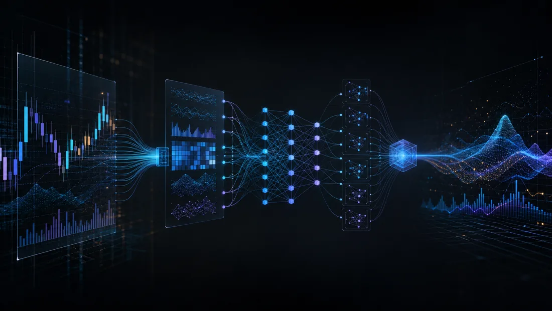
This blog has spent a long arc on how to search: which sampler to use and when (the crossover is eval cost), how to price the search you ran (the Deflated Sharpe Ratio), how to score the selection procedure itself (PBO), and where that whole apparatus honestly lands (no robust edge).
ما لم يتم تغطيته مطلقًا هو ما تبحث عنه أكثر. تأخذ جميع هذه المقالات مجموعة الميزات وعائلة الإستراتيجية كما هي وتعمل على تحسين المعلمات بداخلها. يقوم AutoML بمهاجمة الطبقة أعلاه — فهو يعمل على أتمتة إنشاء المرشحين أنفسهم. ثلاثة أجزاء من ذلك لا تظهر في أي مكان آخر في هذه المدونة:
- الاستخراج التلقائي للميزات — يقوم بتحويل سلسلة أسعار واحدة إلى ما يقرب من 794 ميزة مميزة إحصائيًا، وتقوم أدوات الميزات بتكوين الميزات عبر جداول السوق ذات الصلة عبر التوليف العميق للميزات.
- AutoML المراعي للميزانية — تحسين التكلفة من FLAML، والذي يجد أفضل نموذج ضمن ميزانية حسابية بدلاً من بغض النظر عن التكلفة.
- مصنع ألفا الصيغةي — 101 صيغة ألفا من WorldQuant باعتبارها قواعد نحوية قابلة للتركيب يمكن للآلة تعدادها.
كل شيء آخر - الوظيفة الموضوعية، ونظام التحقق من الصحة، وتصحيح الاختبارات المتعددة - تم قياسه بالفعل في مكان آخر هنا، لذا فإن هذه المقالة تربط بدلاً من إعادة التدريس. هذا مهم أكثر من المعتاد، لأن AutoML يجعل عدد التجارب ينفجر، وعدد التجارب هو بالضبط ما تدور حوله بقية القوس.
! ZXQKEEP0QXZ
ما الذي يقوم بأتمتة AutoML
AutoML ليس خوارزمية واحدة. إنها مجموعة من التقنيات التي تعمل على أتمتة مراحل مختلفة من خط الأنابيب:
| المرحلة | النهج اليدوي | نهج AutoML |
|---|---|---|
| هندسة مميزة | مؤشرات مجال الحرف الخبيرة | الاستخراج الآلي (tsfresh، أدوات الميزات) |
| اختيار الميزة | تحليل الارتباط والحدس | اختبار الفرضيات الإحصائية، SHAP |
| اختيار النموذج | جرب 2-3 نماذج | البحث في العشرات من المتعلمين |
| ضبط المعلمة الفائقة | بحث الشبكة، التغيير والتبديل اليدوي | بحث بايزي / اقتصادي التكلفة (Optuna، FLAML) |
| التصميم المعماري | طوبولوجيا الشبكة العصبية الثابتة | بحث العمارة العصبية (NAS) |
| بناء الفرقة | التراص اليدوي | اختيار المجموعة الآلي |
الفرضية هي أنه في التداول المنهجي تكون المساحة المرشحة هائلة - سلسلة OHLCV واحدة تولد مئات الميزات التقنية، والأصول المتعددة وبيانات دفتر الطلبات والمصادر البديلة تجعلها اندماجية. وتشكل الفرضية أيضًا خطرًا: كل مرشح هو بمثابة تجربة، والتجارب هي التي تصنع الاكتشافات الكاذبة.
One AutoML-specific point on the objective: the metric the search maximizes must be the financial one, because the search will optimize exactly what you wrote down and nothing you meant. Which scalar you pick silently selects your strategy — see Objective-Function Design, where a naive per-trade Sharpe crowns a sub-5%-exposure lottery in 56% of 600 seeds and posts an in-sample Sharpe of 21 that collapses to 0.13 out of sample. Wire the financial metric into the AutoML scorer from the start; do not optimize roc_auc and hope it transfers.
هندسة الميزات الآلية
هندسة الميزات هي المكان الذي يعيش فيه معظم ألفا. بيانات الأسعار الأولية هي نفسها بالنسبة للجميع. إن تحويل تلك البيانات إلى إشارات تنبؤية هو ما يفصل الاستراتيجيات المربحة عن الضوضاء.
! ZXQKEEP0QXZ
tsfresh: من سلسلة أسعار واحدة إلى أكثر من 800 ميزة
tsfresh (Time Series Feature Extraction based on Scalable Hypothesis Tests) is purpose-built for time series feature extraction. It computes 63 characterization methods that expand into ~794 features by default, including:
- لحظات إحصائية (المتوسط، التباين، الانحراف، التفرطح)
- الارتباط التلقائي في فترات تأخر متعددة
- معاملات فورييه والطاقة الطيفية
- مقاييس التعقيد (الإنتروبيا التقريبية، إنتروبيا العينة)
- الخصائص غير الخطية (معاملات فريدريش، أقصى نقطة ثابتة لانجفين)
- تغيير الكميات وأعداد النطاق
For financial data, this means a single price series produces hundreds of candidate features — many capturing dynamics that manual feature engineering would miss. This is a materially different approach from the hand-crafted, domain-derived feature sets used in spread modeling and DeepLOB: there a human decides that order-book imbalance matters; here a library enumerates everything and lets a hypothesis test decide. For financial data, this means a single price series produces hundreds of candidate features — many capturing dynamics that manual feature engineering would miss. This is a materially different approach from the hand-crafted, domain-derived feature sets used in spread modeling and DeepLOB : there a human decides that order-book imbalance matters; here a library enumerates everything and lets a hypothesis test decide.
import pandas as pd
import numpy as np
from tsfresh import extract_features, select_features
from tsfresh.utilities.dataframe_functions import impute

def prepare_rolling_windows(df: pd.DataFrame, window_size: int = 20) -> pd.DataFrame:
    """Convert OHLCV DataFrame into rolling windows for tsfresh."""
    records = []
    for i in range(window_size, len(df)):
        window = df.iloc[i - window_size:i].copy()
        window["id"] = i  # window identifier
        window["time"] = range(window_size)
        records.append(window[["id", "time", "close", "volume", "high", "low"]])
    return pd.concat(records, ignore_index=True)

df_ohlcv = pd.read_csv("btc_1h.csv", parse_dates=["timestamp"])
df_rolled = prepare_rolling_windows(df_ohlcv, window_size=24)

features = extract_features(
    df_rolled,
    column_id="id",
    column_sort="time",
    n_jobs=8,  # parallel extraction
    disable_progressbar=False,
)

impute(features)

y = df_ohlcv["close"].pct_change(4).shift(-4).iloc[24:].reset_index(drop=True)
y_binary = (y > 0).astype(int)

features_selected = select_features(features, y_binary, fdr_level=0.05)
print(f"Selected {features_selected.shape[1]} features from {features.shape[1]}")
The select_features function applies a Benjamini-Yekutieli procedure to control the false discovery rate across the whole feature battery — which is the right instinct, and the same instinct the Deflated Sharpe article applies to strategy searches. Note what it does not do: FDR control on the feature-selection step says nothing about the trial cost of the model search that follows it. Those are two separate multiplicities and both have to be paid.
أدوات الميزات: التوليف العميق للميزات
While tsfresh focuses on time series characterization, Featuretools excels at relational feature engineering — constructing features by composing primitive operations across related tables.
بالنسبة للتداول، يكون هذا فعالاً عندما يكون لديك بيانات متعددة الجداول: تاريخ التداول، ولقطات دفتر الطلبات، ومعدلات التمويل، والمقاييس الموجودة على السلسلة. تطبق أدوات الميزة ميزة التركيب العميق للميزات (DFS)، التي تقوم بتكديس أساسيات التحويل والتجميع: For trading, this is powerful when you have multi-table data: trade history, order book snapshots, funding rates, and on-chain metrics. Featuretools applies Deep Feature Synthesis (DFS), which stacks transformation and aggregation primitives:
import featuretools as ft

es = ft.EntitySet(id="crypto_trading")

es = es.add_dataframe(
    dataframe_name="candles",
    dataframe=df_candles,
    index="candle_id",
    time_index="timestamp",
)

es = es.add_dataframe(
    dataframe_name="orderbook",
    dataframe=df_orderbook,
    index="snapshot_id",
    time_index="timestamp",
)

es = es.add_dataframe(
    dataframe_name="funding",
    dataframe=df_funding,
    index="funding_id",
    time_index="timestamp",
)

feature_matrix, feature_defs = ft.dfs(
    entityset=es,
    target_dataframe_name="candles",
    agg_primitives=["mean", "std", "max", "min", "skew", "trend"],
    trans_primitives=["percentile", "diff", "cum_mean"],
    max_depth=2,  # compose up to 2 primitives deep
    features_only=False,
)

print(f"Generated {len(feature_defs)} features via DFS")
The time_index declaration is load-bearing: it is what lets Featuretools compute aggregations using only rows that existed at the cutoff. Get it wrong and DFS will happily build a feature out of the future — the relational-data instance of the leaks catalogued in the look-ahead bias taxonomy.
يمنحك الجمع بين tsfresh (توصيف السلاسل الزمنية) وFeaturetools (التوليف العلائقي) مصنعًا للميزات ينتج آلاف الإشارات المرشحة من بيانات السوق الأولية دون الحاجة إلى ترميز يدوي للمؤشر.
AutoML المراعي للميزانية: FLAML
We assume Optuna and Tree-structured Parzen Estimators as background — the derivation, sampler comparison and benchmark are in Coordinate Descent vs Bayesian Optimization. On which sampler to reach for, this blog's own measurement is the reference and it is not the folklore answer: the crossover is governed by evaluation cost, not algorithm cleverness — when a backtest is nearly free, scrambled Sobol wins on throughput (~2,830 cfg/s against ~154 for TPE), and only expensive evaluations make sample efficiency pay (Random vs Smart Search).
! ZXQKEEP0QXZ
That framing is what makes FLAML a different axis rather than a competing sampler. Optuna asks where to sample next; FLAML (Fast Lightweight AutoML) asks what can I afford to sample at all. It optimizes for the best model within a time or compute budget using CFO (Cost-Frugal Optimization), which prioritizes cheap-to-evaluate configurations early and escalates only when the estimated marginal gain justifies the spend. That framing is what makes FLAML a different axis rather than a competing sampler. Optuna asks where to sample next; FLAML (Fast Lightweight AutoML) asks what can I afford to sample at all. It optimizes for the best model within a time or compute budget using CFO (Cost-Frugal Optimization), which prioritizes cheap-to-evaluate configurations early and escalates only when the estimated marginal gain justifies the spend.
from flaml import AutoML
from sklearn.metrics import make_scorer
import numpy as np

def sharpe_score(y_true, y_pred):
    """Custom scorer: Sharpe ratio of predicted signals."""
    signal = np.sign(y_pred - 0.5)
    returns = signal * y_true  # y_true contains forward returns
    if returns.std() == 0:
        return 0.0
    return np.sqrt(252) * returns.mean() / returns.std()

sharpe_scorer = make_scorer(sharpe_score, greater_is_better=True)

automl = AutoML()
automl_settings = {
    "time_budget": 300,          # 5 minutes
    "metric": sharpe_scorer,     # optimize the financial objective, not accuracy
    "task": "classification",
    "estimator_list": [
        "lgbm", "xgboost", "rf", "extra_tree", "catboost",
    ],
    "eval_method": "cv",
    "split_type": "time",        # time series split (no future leakage)
    "n_splits": 5,
    "log_file_name": "flaml_trading.log",
    "seed": 42,
}

automl.fit(
    X_train=X_train,
    y_train=y_train,
    **automl_settings,
)

print(f"Best model: {automl.best_estimator}")
print(f"Best config: {automl.best_config}")

from flaml.data import get_output_from_log
time_history, best_valid_loss_history, valid_loss_history, config_history, metric_history = \
    get_output_from_log(filename="flaml_trading.log", time_budget=300)
ميزة FLAML للتداول هي حساب التخصيص عبر أنواع النماذج غير المتجانسة. إذا تم تقييم تكوينات LightGBM أسرع بـ 10 مرات من CatBoost، فإن FLAML يستكشف المزيد من LightGBM مبكرًا ويقوم بالتبديل فقط عندما يقدر أن التحسين الهامشي يبرر التكلفة. هذه هي رؤية النظام الرخيص من مقالة التقاطع المعممة: الإنتاجية هي مصطلح من الدرجة الأولى في ميزانية البحث، وليست تفاصيل التنفيذ.
سجل المسار هو الجزء الذي يستحق الاحتفاظ به. يمنحك ZXQKEEP0QXZ سجل التكوين الكامل، وهو عدد التجارب الخاصة بك - وعدد التجارب هو المدخل لكل انكماش أنت على وشك أن تدين به.
الهندسة العصبية تبحث عن نماذج التداول
Neural Architecture Search automates the design of network topologies rather than the tuning of a fixed one. Architecture choice for financial series is genuinely non-obvious — non-stationarity, low signal-to-noise, mixed frequencies and dependencies spanning minutes to months all pull in different directions — but that motivation is already argued concretely elsewhere: see Temporal Fusion Transformer on when TFT beats LSTM beats vanilla Transformer, and DeepLOB on the CNN+Inception+LSTM tradeoff, for what carefully hand-designed fixed architectures already achieve. NAS is the argument that this choice should itself be searched.
Research on Neuroevolution NAS for Stock Return Prediction reports that RNNs evolved via EXAMM (Evolutionary eXploration of Augmenting Memory Models) outperformed the DJI and S&P 500 in both bear (2022) and bull (2023) markets using simple long-short strategies. Treat that as a third-party claim, not as a result reproduced here — it is a best-of-search figure with no deflation reported.
مساحة بحث NAS للتجارة
تتضمن مساحة البحث العملية لـ NAS لنماذج التداول ما يلي: A practical NAS search space for trading models includes:
Search Space:
  - Cell types: {LSTM, GRU, Temporal Conv, Transformer block, Linear}
  - Number of layers: [1, 8]
  - Hidden dimensions: {32, 64, 128, 256}
  - Attention heads (if Transformer): {2, 4, 8}
  - Dropout rate: [0.0, 0.5]
  - Skip connections: {True, False}
  - Normalization: {BatchNorm, LayerNorm, None}
  - Activation: {ReLU, GELU, SiLU, Mish}
  - Lookback window: {20, 60, 120, 252}
باستخدام NNI (ذكاء الشبكة العصبية) من Microsoft، يمكنك تحديد هذه المساحة والبحث فيها: With NNI (Neural Network Intelligence) from Microsoft, you can define and search this space:
import nni
from nni.nas.nn.pytorch import LayerChoice, InputChoice
import torch
import torch.nn as nn

class TradingNASModel(nn.Module):
    """NAS-searchable model for financial time series."""

    def __init__(self, input_dim: int, seq_len: int):
        super().__init__()
        self.input_proj = nn.Linear(input_dim, 128)

        self.temporal_block = LayerChoice([
            nn.LSTM(128, 128, num_layers=2, batch_first=True, dropout=0.1),
            nn.GRU(128, 128, num_layers=2, batch_first=True, dropout=0.1),
            nn.TransformerEncoder(
                nn.TransformerEncoderLayer(d_model=128, nhead=4, batch_first=True),
                num_layers=2,
            ),
        ], label="temporal_cell")

        self.head = LayerChoice([
            nn.Sequential(nn.Linear(128, 64), nn.ReLU(), nn.Linear(64, 1)),
            nn.Sequential(nn.Linear(128, 32), nn.GELU(), nn.Linear(32, 1)),
            nn.Linear(128, 1),
        ], label="prediction_head")

        self.skip = InputChoice(n_candidates=2, n_chosen=1, label="skip_conn")
        self.skip_proj = nn.Linear(input_dim, 128)

    def forward(self, x: torch.Tensor) -> torch.Tensor:
        h = self.input_proj(x)
        out = self.temporal_block(h)

        if isinstance(out, tuple):
            out = out[0]

        last = out[:, -1, :]

        skip_val = self.skip_proj(x[:, -1, :])
        last = self.skip([last, last + skip_val])

        return self.head(last).squeeze(-1)
تقوم خوارزمية البحث (ENAS، أو DARTS، أو التطورية) بتقييم البنى المرشحة على مجموعة التحقق من الصحة باستخدام هدف مالي، ثم تضيق تدريجيًا نحو طبولوجيا عالية الأداء. لاحظ عدم تناسق التكلفة مقابل كل شيء آخر في هذه المقالة: يقع NAS في النهاية الباهظة الثمن لمحور تكلفة التقييم، وهو النظام الوحيد الذي تدفع فيه أجهزة أخذ العينات ذات الكفاءة العالية والتشذيب متعدد الدقة تكاليفها بشكل حقيقي.
نهج مصنع WorldQuant Alpha
يعتبر أسلوب WorldQuant في اكتشاف ألفا هو التطبيق الأكثر تطبيقًا على المستوى الصناعي لمبادئ AutoML في مجال التمويل. تدير شركة WorldQuant، التي أسسها إيجور تولشينسكي، ما يسمونه "مصنع ألفا" - وهي عملية منهجية لتوليد واختبار ودمج الملايين من الإشارات التنبؤية.
الفلسفة: توليد ألفا الأسي وتصحيحه
حددت شركة WorldQuant هدفًا في عام 2010 للوصول إلى مليون ألفا، في الوقت الذي كانت تنتج فيه عدة آلاف فقط سنويًا. لقد حققوا هذا الهدف في عام 2016. وترتكز الفلسفة على القانون الأساسي للإدارة النشطة:
ZXQKEEP0QXZ
حيث ZXQKEEP0QXZ هو نسبة المعلومات، وZXQKEEP1QXZ هو معامل المعلومات، وZXQKEEP2QXZ هو العرض - عدد الرهانات المستقلة. كل فرد ZXQKEEP3QXZ هو متنبئ ضعيف؛ الادعاء هو أن الجمع بين ما يكفي من العناصر المترابطة بشكل ضعيف يؤدي إلى تحويل الشهادات المرحلية الصغيرة إلى عائد ذي مغزى معدل حسب المخاطر.
The correction that makes or breaks this, and that the naive reading of the formula hides: breadth is not trial count. counts independent bets, and generated alphas are not independent — they are composed from the same operators over the same price and volume fields, so they inherit each other's correlation structure. This blog measured the effect directly in Signal Correlation: effective breadth is , and with a typical crypto correlation factor , ten signals are worth about 3.3 independent ones. The term does not grow with how many alphas you generated; it grows with how many uncorrelated ones survived. A million correlated alphas buy you far less than the formula advertises.
هذا هو السبب في أن الخطوة 3 أدناه - إلغاء الارتباط بالمكتبة الموجودة - ليست خطوة نظافة في مصنع ألفا. إنها الخطوة التي تنتج الاتساع في المقام الأول.
101 صيغة ألفا
The paper "101 Formulaic Alphas" by Kakushadze (associated with WorldQuant research) published a set of formulaic alpha expressions — mathematical expressions over price, volume and fundamental data: The paper "101 Formulaic Alphas" by Kakushadze (associated with WorldQuant research) published a set of formulaic alpha expressions — mathematical expressions over price, volume and fundamental data:
Alpha#1:  (rank(Ts_ArgMax(SignedPower(((returns < 0) ? stddev(returns, 20)
          : close), 2.), 5)) - 0.5)

Alpha#7:  ((adv20 < volume) ? ((-1 * ts_rank(abs(delta(close, 7)), 60))
          * sign(delta(close, 7))) : (-1 * 1))

Alpha#42: (rank(vwap - close) / rank(vwap + close))
ما يجعل هذا الأمر مثيرًا للاهتمام بالنسبة لـ AutoML هو أنه قواعد نحوية. ألفا عبارة عن تركيبات لمجموعة عوامل صغيرة ( ZXQKEEP0QXZ، ZXQKEEP1QXZ، ZXQKEEP2QXZ، ZXQKEEP3QXZ، ZXQKEEP4QXZ، ZXQKEEP5QXZ) على مجموعة حقول صغيرة (ZXQKEEP6QXZ، ZXQKEEP7QXZ، ZXQKEEP8QXZ، ZXQKEEP9QXZ، ZXQKEEP10QXZ). القواعد النحوية قابلة للتعداد، مما يعني أن مساحة البحث قابلة للإنشاء آليًا بطريقة لا تكون كذلك "التفكير في ميزة جيدة". يمكن لنظام AutoML:
- إنشاء التعبيرات المرشحة عن طريق تركيب عوامل التشغيل على حقول البيانات
- تقييم IC لكل تعبير، ومعدل دورانه، وسحبه
- تصفية للتعبيرات التي تصمد أمام الاختبارات الإحصائية و غير المرتبطة بشكل كافٍ بالمكتبة الحالية
- اجمع الناجين في محفظة
لاحظ أن الخطوتين 1 و2 هما الخطوتان السهلتان والخطوة 3 هي حيث القيمة - راجع تصحيح الاتساع أعلاه.
اكتشاف ألفا المعزز LLM
WorldQuant has begun integrating large language models into the alpha factory. As reported in financial press, the firm is exploring how LLMs can "transform and discover alphas across different domains" — generating novel expressions, translating research papers into testable hypotheses, and surfacing cross-domain relationships that a pure enumerative search would miss. This is a different mechanism from extracting signals from text, which this blog covers in LLM Alpha Mining on Earnings Calls; here the LLM writes the formula, not the feature.
قم ببناء مصنع Mini Alpha الخاص بك
فيما يلي مصنع ألفا مدمج ولكنه عملي فوق قواعد المشغل: Here is a compact but functional alpha factory over the operator grammar:
import itertools
from dataclasses import dataclass
from typing import Callable, List
import pandas as pd
import numpy as np
from scipy.stats import spearmanr

@dataclass
class Alpha:
    name: str
    expression: Callable[[pd.DataFrame], pd.Series]
    ic: float = 0.0
    turnover: float = 0.0
    sharpe: float = 0.0

def ts_rank(series: pd.Series, window: int) -> pd.Series:
    return series.rolling(window).apply(lambda x: pd.Series(x).rank().iloc[-1] / len(x))

def ts_delta(series: pd.Series, period: int) -> pd.Series:
    return series.diff(period)

def ts_std(series: pd.Series, window: int) -> pd.Series:
    return series.rolling(window).std()

def cs_rank(series: pd.Series) -> pd.Series:
    return series.rank(pct=True)

def ts_mean(series: pd.Series, window: int) -> pd.Series:
    return series.rolling(window).mean()

ALPHA_TEMPLATES = [
    ("momentum_{w}",
     lambda df, w: cs_rank(ts_delta(df["close"], w))),
    ("mean_reversion_{w}",
     lambda df, w: -cs_rank(df["close"] / ts_mean(df["close"], w) - 1)),
    ("vol_surprise_{w}",
     lambda df, w: cs_rank(df["volume"] / ts_mean(df["volume"], w))),
    ("price_vol_divergence_{w}",
     lambda df, w: cs_rank(ts_delta(df["close"], w)) * -cs_rank(ts_delta(df["volume"], w))),
    ("volatility_rank_{w}",
     lambda df, w: -cs_rank(ts_std(df["close"].pct_change(), w))),
    ("high_low_range_{w}",
     lambda df, w: cs_rank(ts_mean(df["high"] - df["low"], w) / df["close"])),
]

WINDOWS = [5, 10, 20, 60, 120]

def generate_alphas(df: pd.DataFrame, forward_returns: pd.Series) -> List[Alpha]:
    """Generate and evaluate all alpha candidates."""
    alphas = []

    for (name_tpl, expr_fn), window in itertools.product(ALPHA_TEMPLATES, WINDOWS):
        name = name_tpl.format(w=window)
        try:
            signal = expr_fn(df, window)
            signal = signal.replace([np.inf, -np.inf], np.nan)

            valid = signal.notna() & forward_returns.notna()
            if valid.sum() < 100:
                continue

            ic, _ = spearmanr(signal[valid], forward_returns[valid])
            turnover = signal.diff().abs().mean()

            ret = (signal * forward_returns).dropna()
            sharpe = np.sqrt(252) * ret.mean() / (ret.std() + 1e-9)

            alphas.append(Alpha(
                name=name,
                expression=lambda df, fn=expr_fn, w=window: fn(df, w),
                ic=ic,
                turnover=turnover,
                sharpe=sharpe,
            ))
        except Exception:
            continue

    alphas.sort(key=lambda a: abs(a.ic), reverse=True)
    return alphas
ستة قوالب على خمس نوافذ عبارة عن عملية مسح مكونة من 30 تكوينًا. يحتوي التقرير الذي يصدره على هذا الشكل التخطيطي — الحقول هي ما ينبعث من المصنع، ولا يتم ملء أي أرقام لأنه لم يتم قياس أي منها هنا: Six templates over five windows is a 30-configuration sweep. The report it produces has this schematic shape — the fields are what the factory emits, and no numbers are filled in because none have been measured here:
SCHEMATIC — illustrative format only, not a measurement

Generated <N> alphas from <N> candidate configurations

Top by |IC|:
  <alpha_name>   IC=<±0.0xxx>   Sharpe=<±x.xxx>   Turnover=<0.0xxx>
  ...
The raw Sharpe of the top alpha out of a 30-configuration sweep is not a result — it is the maximum of 30 draws, and on 1,000 zero-edge strategies the best annualized Sharpe averages 1.63 while the naive test declares a discovery 100% of the time (Deflated Sharpe Ratio). The honest deliverable from a factory is therefore not "we found an alpha" but how many alphas survived deflation: the IC distribution, the trial count, the winner's DSR against that count, and the PBO of the selection. That is the measurement this section still owes.
حواجز الحماية: ما تدين به بالفعل
يعمل AutoML على تضخيم الاكتشاف والتركيب الزائد على قدم المساواة، ويفعل ذلك عند عدد التجارب حيث لا يكون الفرق دقيقًا. يتم تناول كل واحدة منها بعمق في مكان آخر؛ النقطة هنا هي أن AutoML يجعلها كلها إلزامية وليست مستحسنة.
Price the search, do not merely correct it. A feature-model-hyperparameter sweep is a trial count and the trial count moves the bar — see The Deflated Sharpe Ratio.
Validate temporally, with purging and embargo. See Walk-Forward Optimization and the Look-Ahead Bias Taxonomy for the leaks that survive a naive temporal split.
Score the procedure, not just the winner. See Probability of Backtest Overfitting, and carry its load-bearing correction: PBO's null is 0.5, not 1 — half is not "half overfit," it is fully overfit, a coin flip.
Watch for peaks that are not there. Searching a noise-dominated surface efficiently just finds sharper illusions faster (Plateau Analysis); this bites hardest on strategy parameters and least on ML hyperparameters, which is the case FLAML and Optuna are actually built for.
تقييد مساحة البحث. الحد الأدنى لعينات الأوراق، والحد الأقصى للعمق وعدد التقديرات، وميزانية الميزات، وعقوبة دوران - تنظيم البحث أرخص من تفريغه بعد ذلك.
الخلاصة
يقوم AutoML بنقل الأتمتة إلى مستوى أعلى: من ضبط المعلمات داخل مرشح ثابت إلى إنشاء المرشحين أنفسهم. هناك ثلاثة مكونات تستحق الجهد المبذول - tsfresh وFeaturetools لإنشاء الميزات، وبحث FLAML المقتصد من حيث التكلفة لاختيار النموذج المراعي للميزانية، والقواعد النحوية للمشغل لبناء ألفا لا يحصى. تصبح NAS تستحق الحوسبة فقط عندما تبررها نسبة الإشارة إلى الضوضاء، وتعيش عند الطرف المكلف من محور تكلفة التقييم حيث يتم دفع كفاءة العينة في النهاية.
تبقى وسيطة اتساع WorldQuant على قيد الحياة مع قياسات هذه المدونة الخاصة فقط في شكلها المصحح: ZXQKEEP0QXZ حيث يقوم ZXQKEEP1QXZ بحساب الرهانات المستقلة، ولا يقترب إنتاج المصنع من الاستقلال بأي حال من الأحوال. توليد مليون ألفا هو النصف السهل. إثبات أنها غير مترابطة بما يكفي لاعتبارها اتساعًا هو النصف الذي يحدد ما إذا كانت الصيغة تعني أي شيء.
And the honest caveat is not a moral, it is a measured result. This blog ran the search-and-overfit arc to its conclusion in The Honest Negative: tens of thousands of backtests across five majors, DSR = 0.00 at ~37,000 trials, PBO 0.264 and 0.327, and no robust edge. AutoML raises the trial count by orders of magnitude. Whatever it finds, it will owe a correspondingly larger deflation — and the useful output of an alpha factory is the survival rate after that deflation, not the top line before it. And the honest caveat is not a moral, it is a measured result. This blog ran the search-and-overfit arc to its conclusion in The Honest Negative : tens of thousands of backtests across five majors, DSR = 0.00 at ~37,000 trials, PBO 0.264 and 0.327, and no robust edge. AutoML raises the trial count by orders of magnitude. Whatever it finds, it will owe a correspondingly larger deflation — and the useful output of an alpha factory is the survival rate after that deflation, not the top line before it.
Authors
Trading-systems engineer
Trading-systems engineer building bots since 2017: cross-exchange arbitrage (connected up to 30 venues), cointegration-based pairs arbitrage across spot and futures, scalping, news and sentiment-driven strategies, trend algorithms, and portfolio management and balancing algorithms. Also builds sub-millisecond order execution, big-data warehouses, backtesting engines, AI agents, and trading interfaces (incl. open-source profitmaker.cc). Stack: JS/TS, Python, Rust/Zig/Go, DevOps, backend, frontend, architecture.
Read More

XGBoost for Return Direction: Class Imbalance and Decision Thresholds

التعلم الآلي المزدوج: تقدير معامل السببية بدلاً من التنبؤ بالعوائد