Backtest-live parity: why your bot trades differently from the backtest
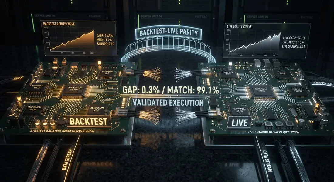
You ran a strategy through a backtest. Sharpe 2.1, MaxDD -8%, PnL +67%. You launched the bot. A month later you compare: the same signals, the same period — but live PnL is 40% lower. The drawdown is one and a half times deeper. Two out of ten trades were not executed at all.
This is not a bug. This is backtest-live divergence — a systematic discrepancy between backtest results and real trading. Everyone has it. The only question is whether you know about it and whether you can control it.
This article provides a complete taxonomy of divergences, architectural patterns for minimizing them, and a practical checklist for monitoring parity in production.
The "it worked in backtest" syndrome

Every algotrader goes through this cycle:
- Wrote a strategy in a Jupyter notebook
- Ran a backtest on historical CSV — results are great
- Rewrote the logic as a bot (often in a different language or framework)
- Launched — results do not match
- Started looking for a bug, did not find one — "the market changed"
The problem is not the market. The problem is that the backtest and the bot are two different software products that model the same reality differently. Divergences are inevitable, but they can be systematized and minimized.
Taxonomy of Divergences

All sources of divergence fall into four categories. For each one — a severity rating (from 1 to 5) and a typical contribution to PnL divergence.
1. Data divergences (severity: 3/5)
The data the backtest sees and the data the bot sees in real time are not the same thing.
Timestamps. Exchanges deliver candles with different rules for timestamp assignment. One exchange marks the candle with the start of the period, another with the end. A REST API may return a candle with a 1-3 second delay after the actual close. The backtest works with "ideal" timestamps from the historical file.
OHLCV aggregation. Historical data is often aggregated by the provider differently than the exchange does in real time. The difference is in the last digit — but with threshold signals (MA crossover, level breakout) this determines whether the strategy enters a position or not.
Gaps and missing data. Historical data is usually clean — missing candles are filled by interpolation. In real time, a WebSocket may drop, and the bot misses 30 seconds of data.
Typical contribution to PnL divergence: 2-5% of annual PnL.
2. Execution divergences (severity: 5/5)

The most dangerous class of divergences. The backtest simulates execution perfectly — reality is far from ideal.
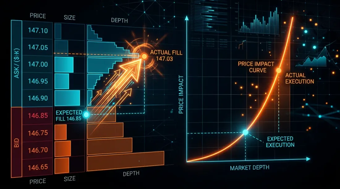
Slippage. The backtest fills the order at the close price (or the signal price). In reality, a market order is executed at the best bid/ask plus slippage that depends on volume and liquidity. For a $10K position on a mid-liquidity altcoin, slippage can be 0.05-0.3%.
Formula for cumulative slippage over trades:
where is the slippage of the -th trade, depending on orderbook depth:
Latency. From the moment a signal is generated to order execution, time passes: signal computation (1-50 ms), request transmission (10-200 ms), matching on the exchange (1-10 ms). In the backtest, latency = 0. In live — the price can move.
Partial fills. The backtest assumes 100% of the order is filled instantly. In reality, a limit order may be partially filled — or not filled at all if the price reverses. For a market order on an illiquid market, the order "slips" through multiple orderbook levels.
Queue priority. A limit order placed at the best bid price will not be filled immediately — it queues behind all previously placed orders at that level. A backtest that considers "price touched = order filled" systematically overstates the fill rate.
Typical contribution to PnL divergence: 10-30% of annual PnL.
3. Logic divergences (severity: 4/5)
These are divergences in the strategy code itself between the backtest and the bot.
Separate codebases. The classic anti-pattern: backtests/strategy_a.py and bot/strategy_a.py — two separate files that "do the same thing." After three months of edits, they inevitably diverge. Someone added a filter in the backtest and forgot to replicate it in the bot. Or the opposite — a bug was fixed in the bot but remained in the backtest.
Different frameworks. Backtest on pandas with vectorized operations, bot on asyncio with event-driven logic. Even with an identical strategy, edge cases are handled differently: rounding, order of condition checks, NaN handling.
State management. The backtest is usually stateless — it iterates over a data array. The bot is stateful — it stores positions, balances, order history. Bot restart, state loss, desynchronization with the exchange — all of these are sources of divergence.
Typical contribution to PnL divergence: 5-20% of annual PnL.
4. Cost divergences (severity: 3/5)
Divergences in trading cost modeling.
Funding rates. Most perpetual futures backtests do not account for funding rates at all. At 10x leverage and an average rate of 0.01% per 8 hours, this is per year — more than the PnL of most strategies. A detailed analysis is in the article Funding rates kill your leverage.
Commissions. Maker/taker commissions are usually modeled but often with the wrong rate. VIP tiers, BNB discounts, rebates — all of these affect the final result.
Spread. A candle-based backtest does not see the bid-ask spread. On a 1-minute candle, close = 3000, but in reality bid = 2999.5 and ask = 3000.5. Each trade "costs" half the spread.
Typical contribution to PnL divergence: 5-15% of annual PnL.
Cumulative Effect
All four categories act simultaneously and, as a rule, in one direction — against the trader:
A total divergence of 20-50% from backtest PnL is normal for an unrefined system. With leverage, the effect is multiplied.
Architectural Patterns for Parity
Pattern 1: Shared Core (extracting a common core)

The idea: extract the strategy core — signal generation and execution logic — into a separate module used by both the backtest and the bot. Only the surrounding infrastructure differs: the data source and the order submission mechanism.
┌─────────────────────────────────────┐
│         strategy_core.py            │
│  ┌─────────────┐ ┌───────────────┐  │
│  │ SignalEngine │ │ OrderManager  │  │
│  └──────┬──────┘ └──────┬────────┘  │
│         │               │           │
│    generate_signal()  create_order()│
└─────────┬───────────────┬───────────┘
          │               │
    ┌─────┴─────┐   ┌─────┴──────┐
    │ Backtest   │   │ Live       │
    │ DataFeed   │   │ DataFeed   │
    │ FillModel  │   │ Exchange   │
    └────────────┘   └────────────┘
from dataclasses import dataclass
from typing import Optional
import numpy as np

@dataclass
class Signal:
    side: str          # 'long' | 'short'
    entry_price: float
    sl_price: float
    tp_price: float
    size: float
    timestamp: int

@dataclass
class OrderRequest:
    side: str
    order_type: str    # 'market' | 'limit'
    price: float
    size: float

class StrategyCore:
    """
    Strategy core. Identical code for backtest and live.
    Depends only on data, not on infrastructure.
    """
    def __init__(self, params: dict):
        self.fast_period = params.get('fast_ma', 20)
        self.slow_period = params.get('slow_ma', 50)
        self.sl_pct = params.get('sl_pct', 0.02)
        self.tp_pct = params.get('tp_pct', 0.04)
        self.position: Optional[Signal] = None
        self._closes: list[float] = []

    def on_candle(self, timestamp: int, o: float, h: float,
                  l: float, c: float, v: float) -> Optional[OrderRequest]:
        """
        Process a new candle. Returns an OrderRequest or None.
        This method is called identically from the backtest and the bot.
        """
        self._closes.append(c)

        if len(self._closes) < self.slow_period:
            return None

        fast_ma = np.mean(self._closes[-self.fast_period:])
        slow_ma = np.mean(self._closes[-self.slow_period:])

        if self.position is not None:
            exit_order = self._check_exit(h, l, c)
            if exit_order:
                self.position = None
                return exit_order

        if self.position is None:
            if fast_ma > slow_ma and self._prev_fast_ma <= self._prev_slow_ma:
                self.position = Signal(
                    side='long', entry_price=c,
                    sl_price=c * (1 - self.sl_pct),
                    tp_price=c * (1 + self.tp_pct),
                    size=1.0, timestamp=timestamp,
                )
                return OrderRequest('buy', 'market', c, 1.0)

        self._prev_fast_ma = fast_ma
        self._prev_slow_ma = slow_ma
        return None

    def _check_exit(self, high: float, low: float,
                    close: float) -> Optional[OrderRequest]:
        pos = self.position
        if pos.side == 'long':
            if low <= pos.sl_price:
                return OrderRequest('sell', 'market', pos.sl_price, pos.size)
            if high >= pos.tp_price:
                return OrderRequest('sell', 'market', pos.tp_price, pos.size)
        return None
Now the backtest and the bot use the same StrategyCore:
from strategy_core import StrategyCore

def run_backtest(candles, params, fill_model):
    core = StrategyCore(params)
    trades = []

    for candle in candles:
        order = core.on_candle(
            candle['timestamp'], candle['open'], candle['high'],
            candle['low'], candle['close'], candle['volume'],
        )
        if order:
            fill_price = fill_model.simulate_fill(order, candle)
            trades.append({'price': fill_price, 'side': order.side})

    return trades
from strategy_core import StrategyCore

async def run_live(exchange, symbol, params):
    core = StrategyCore(params)

    async for candle in exchange.stream_candles(symbol, '1m'):
        order = core.on_candle(
            candle['timestamp'], candle['open'], candle['high'],
            candle['low'], candle['close'], candle['volume'],
        )
        if order:
            await exchange.place_order(symbol, order.side,
                                       order.order_type, order.size)
The key rule: StrategyCore does not know where data comes from or where orders are sent. It receives OHLCV and returns an OrderRequest. Everything else is the responsibility of the infrastructure layer.
Pattern 2: Event-driven unification (NautilusTrader approach)

NautilusTrader implements parity through a unified NautilusKernel — a Rust-native engine with a deterministic event-driven core and nanosecond resolution. The same strategy implementation works in both the backtest and live trading.
The architecture is built on the ports and adapters pattern (hexagonal architecture):
┌──────────────────────────────────┐
│        NautilusKernel            │
│  ┌───────────┐  ┌─────────────┐  │
│  │ Strategy   │  │ RiskEngine  │  │
│  │ (Python)   │  │ (Rust)      │  │
│  └─────┬─────┘  └──────┬──────┘  │
│        │               │         │
│  ┌─────┴───────────────┴──────┐  │
│  │      Message Bus (Rust)    │  │
│  └─────┬───────────────┬──────┘  │
└────────┼───────────────┼─────────┘
         │               │
   ┌─────┴─────┐   ┌─────┴──────┐
   │ Backtest   │   │ Live       │
   │ Adapter    │   │ Adapter    │
   │ FillModel  │   │ Exchange   │
   │ (L2 book)  │   │ Gateway    │
   └────────────┘   └────────────┘
Advantages:
- Deterministic replay. Events are processed in a strictly defined order — the backtest result is bit-reproducible.
- Custom FillModel. L2 orderbook simulation for every execution — slippage is simulated based on real orderbook depth.
- Performance. Up to 5 million rows/sec, processing data that does not fit in RAM.
- Redis + PostgreSQL. Cache and message bus via Redis, persistence via PostgreSQL — identical infrastructure for backtest and live.
Pattern 3: Strategy Interface (Freqtrade approach)
Freqtrade uses a unified IStrategy interface: the same strategy class works in both the backtest and live. The only difference is the persistence layer.
class IStrategy:
    """Unified interface — the implementation does not know if this is a backtest or live."""

    def populate_indicators(self, dataframe, metadata):
        """Compute indicators."""
        dataframe['fast_ma'] = dataframe['close'].rolling(20).mean()
        dataframe['slow_ma'] = dataframe['close'].rolling(50).mean()
        return dataframe

    def populate_entry_trend(self, dataframe, metadata):
        """Determine entry signals."""
        dataframe.loc[
            (dataframe['fast_ma'] > dataframe['slow_ma']) &
            (dataframe['fast_ma'].shift(1) <= dataframe['slow_ma'].shift(1)),
            'enter_long'
        ] = 1
        return dataframe

    def populate_exit_trend(self, dataframe, metadata):
        """Determine exit signals."""
        dataframe.loc[
            (dataframe['fast_ma'] < dataframe['slow_ma']),
            'exit_long'
        ] = 1
        return dataframe
Freqtrade additionally provides:
- Hyperopt via Optuna — strategy parameter optimization
--timeframe-detail— drill-down to a finer timeframe for fill refinement (similar to adaptive drill-down)
Pattern Comparison
| Shared Core | Event-driven (NautilusTrader) | Strategy Interface (Freqtrade) | |
|---|---|---|---|
| Implementation complexity | Low | High | Medium |
| Parity level | Medium | Maximum | High |
| Fill simulation | Separate FillModel | L2 orderbook | --timeframe-detail |
| Core language | Python | Rust + Python | Python |
| Suitable for | Custom engines | Institutional trading | Quick start |
Fill Simulation Accuracy
Fill simulation is the main source of execution divergence. Three levels of accuracy:
Level 1: Naive (fill at close price)
fill_price = candle['close']
Error: does not account for slippage, spread, or partial fills. Systematically overstates PnL.
Level 2: Slippage model
def simulate_fill(order, candle, slippage_bps=5):
    """Fill with slippage."""
    base_price = candle['close']
    slip = base_price * slippage_bps / 10000

    if order.side == 'buy':
        return base_price + slip  # Buy at a higher price
    else:
        return base_price - slip  # Sell at a lower price
Error: fixed slippage does not account for liquidity and order size. Better than naive, but still a crude model.
Level 3: Adaptive drill-down with 1s/100ms data
The best option: use real fine-granularity data for precise determination of SL/TP fill order. Described in detail in the article Adaptive drill-down: backtesting with variable granularity.
class RealisticFillModel:
    """
    Combined fill model: slippage + spread + volume impact.
    """
    def __init__(self, avg_spread_bps=3, impact_coeff=0.1):
        self.avg_spread_bps = avg_spread_bps
        self.impact_coeff = impact_coeff

    def simulate_fill(self, order, candle, order_size_usd):
        base_price = candle['close']

        spread_cost = base_price * self.avg_spread_bps / 20000

        candle_volume_usd = candle['volume'] * candle['close']
        participation_rate = order_size_usd / max(candle_volume_usd, 1)
        impact = base_price * self.impact_coeff * np.sqrt(participation_rate)

        if order.side == 'buy':
            return base_price + spread_cost + impact
        else:
            return base_price - spread_cost - impact
Market impact formula (simplified Almgren-Chriss model):
where is volatility, is the impact coefficient, is the order volume, and is the market volume for the period.
Practical Parity Checklist

Before launching the bot live, verify each item:
Code:
- Strategy uses a shared core (one module for backtest and live)
- No duplication of signal logic in two places
- Unit tests verify identical core outputs for identical inputs
- Order of condition checks is identical (SL before TP? TP before SL?)
Data:
- Timestamp format is identical (UTC, same provider)
- OHLCV aggregation uses the same rules
- Missing candle handling is identical
- No look-ahead bias — the backtest does not peek into the future
Execution:
- Slippage model is calibrated on real data
- Partial fills are modeled (or at least pessimistically estimated)
- Limit orders have a queue priority model
- Latency is accounted for (100-500 ms delay from signal to fill)
Costs:
- Maker/taker commissions are included with the current rate
- Funding rates are accounted for with perpetual futures
- Spread is modeled (at least the average)
Infrastructure:
- State persistence: the bot recovers positions after restart
- Reconnection logic: WebSocket reconnects without data loss
- Logging: all orders and fills are logged for post-mortem analysis
Monitoring Divergence in Production
Parity is not a one-time check but a continuous process. After launching the bot, divergences must be tracked in real time.
Shadow mode (paper trading)

Run the bot in parallel with the backtest on the same data. The bot generates signals but does not send orders — it only logs. Simultaneously, the backtest processes the same data. Compare:
class DivergenceMonitor:
    """
    Compares backtest and live bot signals in real time.
    """
    def __init__(self, tolerance_pct=0.5):
        self.tolerance = tolerance_pct / 100
        self.divergences = []

    def compare_signal(self, backtest_signal, live_signal, timestamp):
        """Compare backtest and live signals."""
        if backtest_signal is None and live_signal is None:
            return  # Both silent — OK

        if (backtest_signal is None) != (live_signal is None):
            self.divergences.append({
                'timestamp': timestamp,
                'type': 'signal_mismatch',
                'backtest': backtest_signal,
                'live': live_signal,
                'severity': 'HIGH',
            })
            return

        price_diff = abs(
            backtest_signal.entry_price - live_signal.entry_price
        ) / backtest_signal.entry_price

        if price_diff > self.tolerance:
            self.divergences.append({
                'timestamp': timestamp,
                'type': 'price_divergence',
                'diff_pct': price_diff * 100,
                'severity': 'MEDIUM',
            })

    def compare_fill(self, backtest_fill, live_fill, timestamp):
        """Compare execution."""
        if backtest_fill and live_fill:
            slippage = (live_fill['price'] - backtest_fill['price']
                        ) / backtest_fill['price']
            self.divergences.append({
                'timestamp': timestamp,
                'type': 'fill_divergence',
                'slippage_bps': slippage * 10000,
                'severity': 'LOW' if abs(slippage) < 0.001 else 'MEDIUM',
            })

    def report(self):
        """Weekly divergence report."""
        from collections import Counter
        severity_counts = Counter(d['severity'] for d in self.divergences)
        return {
            'total_divergences': len(self.divergences),
            'by_severity': dict(severity_counts),
            'avg_slippage_bps': np.mean([
                d['slippage_bps'] for d in self.divergences
                if d['type'] == 'fill_divergence'
            ]) if any(d['type'] == 'fill_divergence'
                      for d in self.divergences) else 0,
        }
Dashboard Metrics
| Metric | Formula | Alert Threshold |
|---|---|---|
| Signal match rate | < 95% | |
| Avg slippage | (bps) | > 10 bps |
| Fill rate | < 90% | |
| PnL divergence | > 20% | |
| Latency p99 | 99th percentile signal-to-fill | > 500 ms |
Slippage Model Calibration
After accumulating data for 2-4 weeks, you can calibrate the backtest slippage model on real data:
def calibrate_slippage(live_fills: list[dict]) -> dict:
    """
    Calibrate slippage model using real fills.

    live_fills: [{'expected_price': ..., 'actual_price': ..., 'size_usd': ..., 'volume_usd': ...}]
    """
    slippages = []
    participation_rates = []

    for fill in live_fills:
        slip = abs(fill['actual_price'] - fill['expected_price']
                   ) / fill['expected_price']
        part = fill['size_usd'] / max(fill['volume_usd'], 1)
        slippages.append(slip)
        participation_rates.append(part)

    slippages = np.array(slippages)
    participation_rates = np.array(participation_rates)

    from scipy.optimize import curve_fit

    def model(x, k, base):
        return k * np.sqrt(x) + base

    popt, _ = curve_fit(model, participation_rates, slippages,
                        p0=[0.1, 0.0001])

    return {
        'impact_coeff': popt[0],
        'base_slippage': popt[1],
        'mean_slippage_bps': np.mean(slippages) * 10000,
        'p95_slippage_bps': np.percentile(slippages, 95) * 10000,
    }
Connections with Other Tools
Backtest-live parity is not an isolated task. It intersects with other tools from the "Backtests Without Illusions" series:
- Adaptive drill-down — improves fill simulation accuracy, a key component of execution parity.
- Funding rates — if the backtest does not model funding, parity is impossible at leverage > 3x.
- Parquet cache — precomputed timeframes and indicators ensure that the backtest sees the same data as the bot. RunningCandleBuffer emulation = real-time updating.
- Polars vs Pandas — when switching from pandas (backtest) to Polars (live), you need to ensure that numerical results match.
- Walk-Forward — walk-forward on out-of-sample data shows how the strategy degrades — this is closer to live than an in-sample backtest.
Recommendations
-
Shared core is mandatory. A single codebase for signal generation is the minimum requirement for parity. Two files with identical logic guarantee divergence within a month.
-
Calibrate the fill model. A fixed 5 bps slippage is better than nothing. A slippage model calibrated on real data is significantly better.
-
Use shadow mode for the first 2-4 weeks. Do not trade with real money until the signal match rate reaches 95%+.
-
Model funding rates. For perpetual futures, this is not optional — it is mandatory. Funding can consume all PnL at leverage > 5x.
-
Log everything. Every signal, every order, every fill — with timestamps. Without logs, post-mortem analysis is impossible.
-
Automate the comparison. A weekly DivergenceMonitor report should arrive automatically. Do not wait until PnL goes negative.
-
Pessimistic backtest by default. It is better to underestimate expectations in the backtest and be pleasantly surprised in live than the reverse. The slippage model should be conservative.
Conclusion

Backtest-live parity is not a property of a system but a process. Perfect parity does not exist: a backtest is by definition a model of reality, and a model always simplifies. But the difference between "the model differs by 5%" and "the model differs by 50%" is determined by architecture.
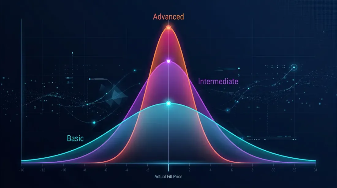
Three levels of maturity:
- Basic. Shared core, fixed slippage, commissions. Divergence: 10-20%.
- Advanced. Event-driven architecture, adaptive drill-down, funding model, shadow mode. Divergence: 5-10%.
- Institutional. L2 orderbook simulation, calibrated impact model, real-time divergence monitoring. Divergence: 2-5%.
Your task is to determine what level you are at and to understand what divergence you consider acceptable for your position size and leverage.
Useful Links
- NautilusTrader — High-Performance Algorithmic Trading Platform
- Freqtrade — Free, open source crypto trading bot
- Almgren, R., Chriss, N. — Optimal Execution of Portfolio Transactions (2001)
- Lopez de Prado — Advances in Financial Machine Learning, Chapter 12: Backtesting
- Ernest Chan — Quantitative Trading: How to Build Your Own Algorithmic Trading Business
- Hexagonal Architecture (Ports and Adapters) — Alistair Cockburn
- Optuna — Hyperparameter Optimization Framework
Citation
@article{soloviov2026backtestliveparity,
  author = {Soloviov, Eugen},
  title = {Backtest-live parity: why your bot trades differently from the backtest},
  year = {2026},
  url = {https://marketmaker.cc/ru/blog/post/backtest-live-parity},
  description = {Complete taxonomy of divergences between backtesting and live trading: from slippage and partial fills to codebase desynchronization. Architectural patterns for achieving parity and a production monitoring checklist.}
}
MarketMaker.cc Team
Quantitative Research & Strategy
Read More

PnL by Active Time: The Metric That Changes Strategy Rankings

Adaptive Drill-Down: Backtest with Variable Granularity from Minutes to Raw Trades