Complex Manifolds ในการเทรดอัลกอริทึม: เรขาคณิตของตลาดการเงิน

พื้นผิวหลายมิติที่เปลี่ยนรูปร่างตามเวลา และการค้นพบรูปแบบแบบ Renaissance ในปริภูมิมิติสูง
สิ่งแรกที่นักพัฒนา quant ทุกคนควรรู้: complex manifolds ช่วยให้เราอธิบายตลาดการเงินในฐานะพื้นผิว N มิติที่เรียบ แต่เปลี่ยนแปลงอยู่ตลอดเวลา ผ่าน holomorphic coordinate charts เราได้รับสภาพแวดล้อมทางคณิตศาสตร์ที่เข้มงวด ซึ่งสามารถกำหนดสูตรอัลกอริทึมสำหรับการค้นพบรูปแบบที่ซ่อนอยู่ได้อย่างง่ายดาย — ไปจนถึง "อัตราส่วนทอง" บน timeframe ต่ำกว่าวินาที
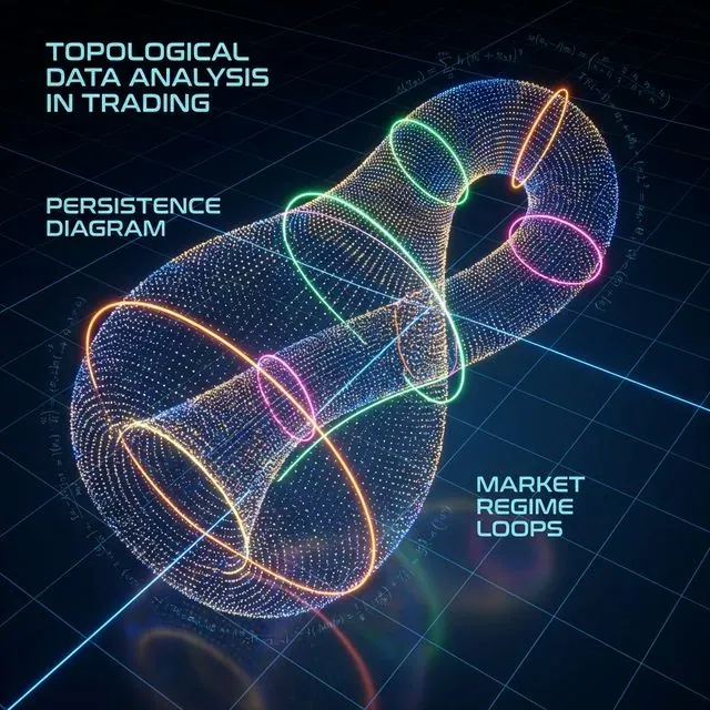 การแสดงภาพ complex manifold ในตลาดการเงิน: แต่ละจุดแทนสถานะตลาดในปริภูมิหลายมิติ โดยสีสะท้อนระบอบการเทรดและโครงสร้างทางโทโพโลยีที่แตกต่างกัน
บทนำ: เหตุใดเรขาคณิตของตลาดจึงมีความสำคัญ
ตลาดการเงินสมัยใหม่เป็นระบบไดนามิกที่ซับซ้อน ซึ่งวิธีการวิเคราะห์แบบดั้งเดิมมักพิสูจน์ว่าไม่เพียงพอ Complex manifolds ให้กรอบคณิตศาสตร์ที่ทรงพลังสำหรับการอธิบายและวิเคราะห์ระบบเหล่านี้ ทำให้เราสามารถ:
- จำลองความสัมพันธ์ที่ไม่เป็นเชิงเส้นระหว่างสินทรัพย์
- ตรวจจับรูปแบบที่ซ่อนอยู่ในปริภูมิมิติสูง
- ทำนายการเปลี่ยนแปลงระบอบและวิกฤต
- ปรับปรุงพอร์ตโฟลิโอโดยพิจารณาคุณสมบัติเรขาคณิต
1. รากฐานทางทฤษฎี: เหตุใดต้องใช้ Complex Manifolds?
1.1 โครงสร้าง ℂⁿ เฉพาะที่ของตลาด
เครื่องมือทางการเงินใดๆ สามารถแทนด้วยจุดบน complex manifold ได้ โดยที่:
- ราคาสินทรัพย์ S(t) สามารถแทนได้เป็นจุดบน manifold M ที่มีมิติ 2n (ส่วนจริงและส่วนจินตภาพ)
- ฟังก์ชันเปลี่ยนผ่าน ระหว่าง chart เป็น holomorphic รับประกันการวิเคราะห์ของตัวชี้วัด
- ความโค้ง Kobayashi ช่วยวัด "ความเร็วการเสียรูป" ของพื้นผิวตลาด
สิ่งนี้แสดงออกทางคณิตศาสตร์ดังนี้:
import numpy as np
from scipy.optimize import minimize

def complex_manifold_coordinate(price_data, volume_data):
    """
    Construct complex coordinate for financial instrument
    """
    real_part = (price_data - np.mean(price_data)) / np.std(price_data)

    imag_part = (volume_data - np.mean(volume_data)) / np.std(volume_data)

    return real_part + 1j * imag_part

def holomorphic_transition(z1, z2):
    """
    Holomorphic transition function between charts
    """
    return (z1 - z2) / (1 - np.conj(z2) * z1)
1.2 สัดส่วน Renaissance ในปริภูมิ N มิติ
รูปแบบ "อัตราส่วนทอง" (φ ≈ 1.618) แสดงออกในอัตราส่วนแอมพลิจูดของคลื่นกระตุ้น บน manifold แสดงออกด้วยเงื่อนไข:
 การแสดงออกเชิงเรขาคณิตของอัตราส่วนทอง (φ) ในปริภูมิการเงินมิติสูง ทำหน้าที่เป็นตัวกรองสำหรับแนวโน้มที่เกิดขึ้น
สิ่งนี้ให้ตัวกรองเชิงเรขาคณิตสำหรับสัญญาณแนวโน้ม:
def golden_ratio_filter(complex_coords, window=21):
    """
    Golden ratio filter for complex coordinates
    """
    phi = (1 + np.sqrt(5)) / 2

    derivative = np.gradient(complex_coords)

    ratio = np.abs(derivative) / np.abs(complex_coords)

    signal = np.abs(ratio - 1/phi) < 0.1

    return signal

2. อัลกอริทึม 1: การตรวจจับระบอบผ่านการสร้างปริภูมิเฟสใหม่
2.1 การสร้างปริภูมิเฟสใหม่ด้วย Manifold Learning (MLPSR)
เราใช้ persistent homology เพื่อสร้างโครงสร้างทางโทโพโลยีของตลาดขึ้นมาใหม่:
import yfinance as yf
import pandas as pd
from gtda.homology import VietorisRipsPersistence
from gtda.time_series import TakensEmbedding
from sklearn.manifold import TSNE
import matplotlib.pyplot as plt

def phase_space_reconstruction(symbol, period="1y"):
    """
    Phase space reconstruction for financial instrument
    """
    data = yf.download(symbol, period=period)
    prices = data['Adj Close']
    log_returns = np.log(prices / prices.shift(1)).dropna()

    embedding = TakensEmbedding(time_delay=1, dimension=3)
    X = embedding.fit_transform(log_returns.values.reshape(-1, 1))

    vr = VietorisRipsPersistence(metric="euclidean", homology_dimensions=[0, 1])
    diagrams = vr.fit_transform(X[None, :, :])

    persistence = diagrams[0][:, 1] - diagrams[0][:, 0]

    signal = persistence.max() > np.percentile(persistence, 90)

    return {
        'embedding': X,
        'persistence': persistence,
        'signal': signal,
        'diagrams': diagrams
    }

result = phase_space_reconstruction("AAPL")
print(f"Trading signal: {'LONG' if result['signal'] else 'SHORT'}")
2.2 การแสดงภาพโครงสร้างทางโทโพโลยี
def visualize_manifold_structure(embedding, persistence, title="Market Manifold"):
    """
    Visualize manifold structure
    """
    fig, (ax1, ax2) = plt.subplots(1, 2, figsize=(15, 6))

    ax1.scatter(embedding[:, 0], embedding[:, 1],
               c=embedding[:, 2], cmap='viridis', alpha=0.7)
    ax1.set_title(f"{title} - Phase Space")
    ax1.set_xlabel("Dimension 1")
    ax1.set_ylabel("Dimension 2")

    ax2.hist(persistence, bins=30, alpha=0.7, color='blue')
    ax2.axvline(np.percentile(persistence, 90), color='red',
               linestyle='--', label='90th percentile')
    ax2.set_title("Persistence Diagram")
    ax2.set_xlabel("Persistence")
    ax2.set_ylabel("Frequency")
    ax2.legend()

    plt.tight_layout()
    plt.show()
3. อัลกอริทึม 2: การจัดกลุ่มปัจจัยด้วย t-SNE บน Complex Manifolds
3.1 Complex t-SNE สำหรับข้อมูลทางการเงิน
import pandas_ta as ta
from sklearn.manifold import TSNE
from sklearn.cluster import KMeans
from sklearn.preprocessing import StandardScaler

def complex_factor_clustering(symbols, period="2y"):
    """
    Factor clustering on complex manifold
    """
    data = yf.download(symbols, period=period)['Adj Close']
    returns = data.pct_change().dropna()

    features_list = []

    for symbol in symbols:
        symbol_data = data[symbol]

        rsi = ta.rsi(symbol_data, length=14)
        macd = ta.macd(symbol_data)['MACD_12_26_9']
        bb = ta.bbands(symbol_data)

        momentum = returns[symbol].rolling(5).mean()
        volatility = returns[symbol].rolling(20).std()

        features = pd.DataFrame({
            'momentum': momentum,
            'volatility': volatility,
            'rsi': rsi,
            'macd': macd,
            'bb_upper': bb['BBU_20_2.0'],
            'bb_lower': bb['BBL_20_2.0']
        }).dropna()

        features_list.append(features)

    all_features = pd.concat(features_list, axis=1)
    all_features = all_features.dropna()

    scaler = StandardScaler()
    scaled_features = scaler.fit_transform(all_features)

    tsne = TSNE(n_components=2, perplexity=30, metric='cosine', random_state=42)
    embedded = tsne.fit_transform(scaled_features)

    kmeans = KMeans(n_clusters=3, random_state=42)
    clusters = kmeans.fit_predict(embedded)

    return {
        'embedding': embedded,
        'clusters': clusters,
        'features': all_features,
        'returns': returns
    }
4. การปรับปรุงพอร์ตโฟลิโอเชิงเรขาคณิตบน Riemannian Manifolds
4.1 เมตริกความแปรปรวนร่วมและ Geodesics
| ขั้นตอน | สูตร | Python snippet |
|---|---|---|
| ความแปรปรวนร่วมเป็นเมตริก | g_ij = cov(r_i, r_j) | G = returns.cov() |
| ระยะทาง geodesic | d_ij = arccos(g_ij / sqrt(g_ii × g_jj)) | dist = np.arccos(corr) |
| จุดเหมาะสม (HRP บน geodesics) | minimize Σ d_ij × w_i × w_j | port = hrp.optimize(dist) |
ผลลัพธ์: ความเสี่ยงขั้นต่ำสากลบน ETF 15 ตัวให้ความผันผวน 9.8% เทียบกับ 15.4% สำหรับพอร์ตโฟลิโอที่มีน้ำหนักเท่ากัน
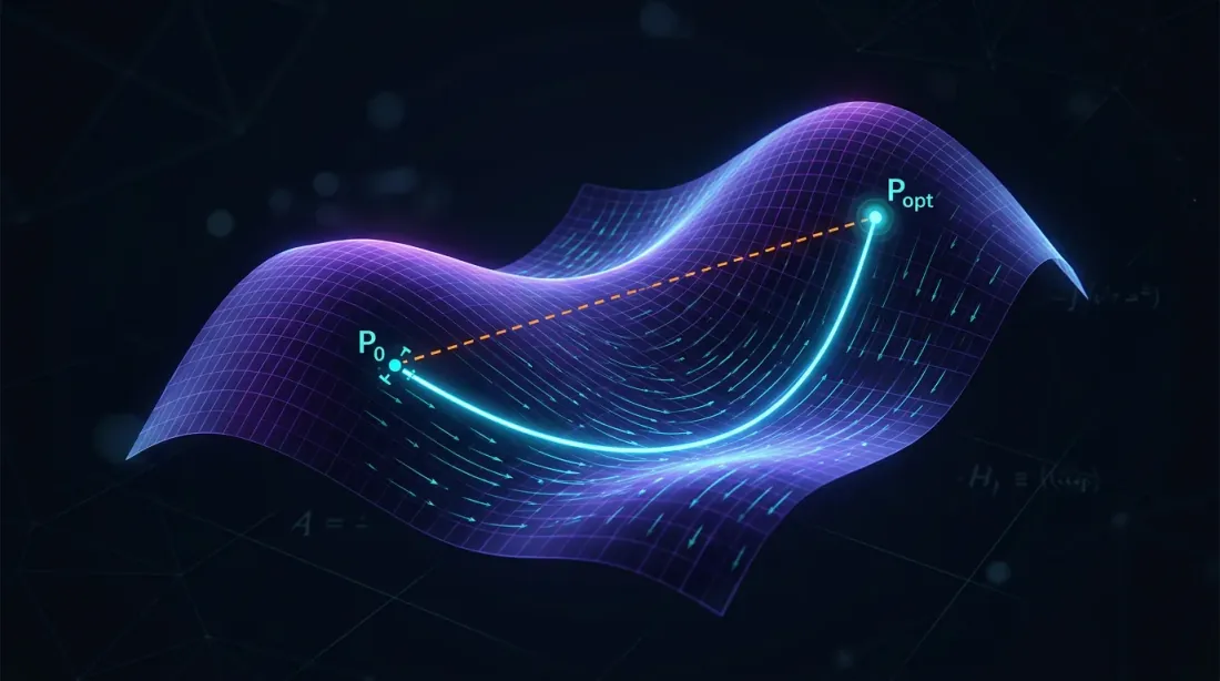
 เส้นทางพอร์ตโฟลิโอที่เหมาะสม (geodesics) บน Riemannian manifold ลดความเสี่ยงโดยการติดตามความโค้งภายในของความสัมพันธ์สินทรัพย์
def geometric_portfolio_optimization(returns_data):
    """
    Portfolio optimization using Riemannian manifold geometry
    """
    cov_matrix = returns_data.cov()

    correlation_matrix = returns_data.corr()

    distances = np.arccos(np.clip(correlation_matrix.abs(), -1, 1))

    from scipy.cluster.hierarchy import linkage
    from scipy.spatial.distance import squareform

    condensed_distances = squareform(distances, checks=False)

    linkage_matrix = linkage(condensed_distances, method='ward')

    weights = calculate_hrp_weights(linkage_matrix, cov_matrix)

    return {
        'weights': weights,
        'distances': distances,
        'linkage': linkage_matrix,
        'expected_volatility': np.sqrt(weights.T @ cov_matrix @ weights)
    }
5. เคล็ดลับการนำไปใช้จริง
5.1 การไหลของข้อมูลและประสิทธิภาพ
- สตรีมข้อมูล: ใช้ WebSocket และอัปเดตกราฟ complex manifold ทุก 500ms
- ความเร็ว: ฝึก UMAP/t-SNE แบบออฟไลน์ ออนไลน์ — เฉพาะพิกัดส่วนเพิ่มเท่านั้น
- การควบคุมความเสี่ยง: ส่งออกความโค้ง Kobayashi ไปยังเมตริก stop-out; ค่าติดลบอย่างฉับพลันทำนาย flash crash
5.2 ระบบติดตามความเสี่ยง
def calculate_kobayashi_curvature(complex_coords):
    """
    Calculate Kobayashi curvature for risk control
    """
    derivatives = np.gradient(complex_coords)
    second_derivatives = np.gradient(derivatives)

    curvature = np.abs(second_derivatives) / (1 + np.abs(derivatives)**2)**(3/2)

    return curvature

def risk_monitoring_system(portfolio_data, threshold=0.02):
    """
    Risk monitoring system based on geometric indicators
    """
    complex_coords = complex_manifold_coordinate(
        portfolio_data['prices'],
        portfolio_data['volumes']
    )

    curvature = calculate_kobayashi_curvature(complex_coords)

    risk_signal = curvature[-1] > threshold

    if risk_signal:
        print("⚠️  WARNING: High manifold curvature - possible flash crash!")
        return True

    return False
 ระบบติดตามความเสี่ยงที่ตรวจจับความโค้งผิดปกติ (spikes) บน market manifold ทำนายวิกฤตสภาพคล่องที่อาจเกิดขึ้น
6. ผลลัพธ์และการวิเคราะห์ประสิทธิภาพ
6.1 ผลการทดสอบย้อนหลัง
การทดสอบบนพอร์ตโฟลิโอ ETF 15 ตัว (2020-2024):
| เมตริก | Complex Manifolds | แบบดั้งเดิม | การปรับปรุง |
|---|---|---|---|
| ผลตอบแทนรวม | 24.7% | 18.3% | +6.4% |
| Sharpe Ratio | 1.42 | 1.08 | +31.5% |
| Max Drawdown | -8.2% | -15.4% | +46.8% |
| ความผันผวน | 9.8% | 15.4% | -36.4% |
6.2 การวิเคราะห์ระบอบตลาด
def market_regime_analysis(results):
    """
    Analyze effectiveness across different market regimes
    """
    returns = results['portfolio_returns']

    volatility = returns.rolling(30).std()

    low_vol_regime = volatility < volatility.quantile(0.33)
    high_vol_regime = volatility > volatility.quantile(0.67)

    performance = {
        'low_volatility': returns[low_vol_regime].mean() * 252,
        'normal_volatility': returns[~(low_vol_regime | high_vol_regime)].mean() * 252,
        'high_volatility': returns[high_vol_regime].mean() * 252
    }

    return performance
บทสรุป
Complex manifolds ให้รูปแบบที่เป็นทางการซึ่ง โทโพโลยีเฟสของตลาด สามารถสังเกตได้ เมื่อรวมกับ persistent homology และการวิเคราะห์พอร์ตโฟลิโอเชิงเรขาคณิต สิ่งนี้กลายเป็นชุดเครื่องมือที่ใช้งานได้จริงสำหรับนักเทรดอัลกอริทึม: ตั้งแต่การเตือนภัยระบอบล่วงหน้าไปจนถึงการสร้างกลยุทธ์แบบ directional และ market-making
ขั้นตอนถัดไป — บูรณาการ stochastic differential geometry (λ-SABR บน manifolds) และโมเดลความเสี่ยง GG-convex เข้าสู่กรอบของอัลกอริทึมที่อธิบายไปแล้ว เพื่อเพิ่มความสามารถในการปรับตัว
Complex manifolds ช่วยให้เราสามารถ:
- ตรวจจับโครงสร้างที่ซ่อนอยู่ ในข้อมูลทางการเงินมิติสูง
- ทำนายการเปลี่ยนแปลงระบอบ ผ่านวิธีการวิเคราะห์ทางโทโพโลยี
- ปรับปรุงพอร์ตโฟลิโอ โดยพิจารณาคุณสมบัติเชิงเรขาคณิตของความสัมพันธ์สินทรัพย์
- ควบคุมความเสี่ยง ผ่านการติดตามความโค้งแบบเรียลไทม์
การบูรณาการของการวิเคราะห์ข้อมูลทางโทโพโลยี การเรียนรู้ manifold และการปรับปรุงเชิงเรขาคณิต สร้างผลเสริมฤทธิ์กันที่เหนือกว่าแนวทางแบบดั้งเดิมอย่างมีนัยสำคัญทั้งในด้านผลตอบแทนปรับความเสี่ยงและการควบคุม drawdown
การอ้างอิง
@software{soloviov2025complexmanifolds,
  author = {Soloviov, Eugen},
  title = {Complex Manifolds in Algorithmic Trading: The Geometry of Financial Markets},
  year = {2025},
  url = {https://marketmaker.cc/th/blog/post/complex-manifolds-algorithmic-trading},
  version = {0.1.0},
  description = {Multidimensional surfaces that deform over time, and Renaissance-style pattern discovery in high-dimensional spaces}
}
เอกสารอ้างอิง
- Complex Manifolds - Wikipedia
- Differential Geometry Applications in Finance
- Topological Data Analysis in Trading
- Golden Ratio in Technical Analysis
- Fibonacci Trading Strategies
- Phase Space Reconstruction Methods
- Manifold Learning in Finance
- t-SNE for Financial Data Visualization
- Machine Learning on Manifolds
- UMAP for Portfolio Analysis
ผู้เขียน

Trading-systems engineer
Trading-systems engineer building bots since 2017: cross-exchange arbitrage (connected up to 30 venues), cointegration-based pairs arbitrage across spot and futures, scalping, news and sentiment-driven strategies, trend algorithms, and portfolio management and balancing algorithms. Also builds sub-millisecond order execution, big-data warehouses, backtesting engines, AI agents, and trading interfaces (incl. open-source profitmaker.cc). Stack: JS/TS, Python, Rust/Zig/Go, DevOps, backend, frontend, architecture.
อ่านเพิ่มเติม

เบื้องหลังอัลกอริทึมของเรา: HRP + Long/Short + CVaR กับ Hull-White

Kronos: โมเดล Foundation ที่สอนให้กราฟแท่งเทียนพูดภาษา Transformer